Continuous From Discrete Transfer Functions

Second order filters are usually implemented digitally by means of recurrence relations of the form

where the coefficients c_j are constants, and the values of x_j and y_j are the jth discrete samples of the input and output functions respectively. The computations are performed once per Δt seconds. Assuming the input and output functions are scaled equally, the coefficients must satisfy the identity

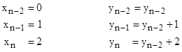
It is often of interest to know how much lag (or lead) such a filter introduces. One way of characterizing this lag is in terms of the asymptotic response to a ramp input. Since the input and output both have constant and equal rates (ultimately), the second-order aspects of the filter drop out, and we effectively have just a first-order lead-lag. To determine the amount of lag, let us assign ramp values to the input and output as follows:

Inserting these into equation (1) we can solve for y_n–2, and since x_n–2 = 0, the value of y_n–2 is the amount by which y differs from x at constant t. Furthermore, since the rate of change of the ramp is 1 unit per iteration, the value of y_n–2 also equals the number of iterations that y leads or lags the ramp input x. Hence if we multiply this by Δt we get the duration of the lag (if the quantity is positive) or lead (if the quantity is negative). Thus we have

For example, suppose we have a second-order digital filter of the form (1) with the coefficients

(Note that these coefficients sum to 1, as required.) Assume the iteration rate of the filter is Δt = 50 msec. Inserting these values into the preceding equation, we find that the filter has a ramp lag of 0.783 seconds.

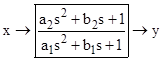
A previous note on Lead-Lag algorithms described how to determine the recurrence coefficients c_j to best represent a continuous second-order transfer function of the form

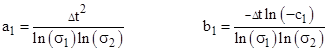
If, instead, we are given the recurrence coefficients and we wish to determine the coefficients of the corresponding continuous transfer function, we immediately have, for the parameters γ and δ from the previous note, γ = –c₁ and δ = c₂. Also, we can compute the denominator coefficients as

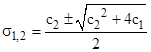
where

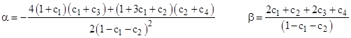
To determine the numerator coefficients, we solve the equations for the optimum second-order recurrence coefficients for the parameters α and β to give

Then we have

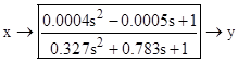
Using the coefficients and iteration interval from the previous example, we get the continuous transfer function shown below.

Thus the filter has essentially no numerator dynamics, and we can confirm from the first-order coefficient in the denominator that this continuous transfer function has a ramp lag of 0.783 seconds, in agreement with what we found earlier for the corresponding discrete digital filter.

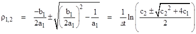
The characteristic roots of the denominator dynamics can be expressed in terms of the coefficients of the continuous transfer function or of the original recurrence relations as

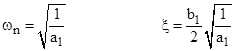
It’s convenient to define the parameters

which are called the natural frequency and the damping ratio respectively. In terms of these parameters the characteristic roots can be written as

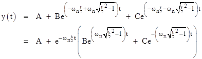
Therefore, the solution y(t) for any fixed input x is of the form

where A, B, C are constants that can be determined from the initial conditions. This shows that the critical value of the damping ratio ξ is 1. For damping ratios greater than 1, the two real exponents are both negative (noting that the square root of ξ² – 1 is necessarily smaller than ξ). Consequently the function y(t) monotonically approaches the fixed value of x. On the other hand, if the damping ratio is less than 1, then for a real solution we must have B = C, and we can express y(t) in terms of the cosine functions as

where

is the damped natural frequency. (We’ve assumed t is defined to give a zero phase angle.) For the numerical example discussed previously, the characteristic roots are

and the solution for any fixed input x is of the form

The exponential factor in the second term has a negative coefficient, so the term approaches zero as time increases. The cosine factor shows that one overshoot cycle lasts for 2π/1.275 = 4.9 units of time.

We can also assess the frequency response of this filter by analyzing the corresponding differential equation

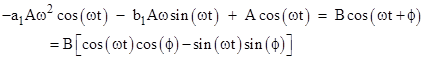
Inserting y(t) = Acos(ωt) and x(t) = Bcos(ωt + ϕ) into this equation, and expanding the latter cosine by means of the angle-addition formula, we get

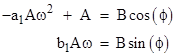
This implies the two relations

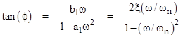
Dividing the second by the first gives the tangent of the phase shift

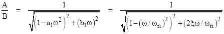
Also, solving for ϕ and inserting into the second of the preceding equations, we can solve for the amplitude ratio A/B, giving

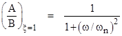
Hence if b₁ is non-zero (meaning that the system has damping) the amplitude ratio is never infinite. For a critically damped system (i.e., with ξ = 1) the amplitude ratio is a Cauchy distribution

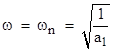
On the other hand, for a totally undamped system (b₁ = ξ = 0), we get an infinite amplitude ratio when

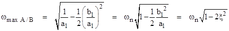
which, as we’ve seen, is the system’s undamped “natural frequency”. For a damped system, i.e., a system with non-zero b₁, the maximum amplitude ratio (for a non-zero frequency) can be found by differentiating the general expression for A/B with respect to ω and setting the result to zero. This gives

as the most responsive frequency. If the damping ratio exceeds 1/√2 the responsiveness drops monotonically as the frequency increases, so there is no real-valued maximum (other than the one at ω = 0).

Return to MathPages Main Menu