Undetected Failures of Threat Protection

Consider a system consisting of two redundant units, each equipped with protection from a common threat (such as lightning, inclement weather, etc), and suppose failure of the protection occurs at the rate r and is undetectable until the unit is subjected to the external threat, at which time the unit fails. In addition, each unit has a detectable failure rate due to generic causes of R, and an exponential repair transition with rate μ. Whenever a unit is repaired, its threat protection is also checked and, if necessary, repaired. Let σ denote the rate of occurrence of the common external threat.

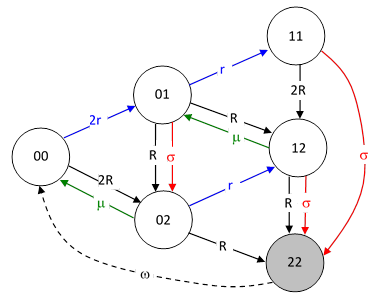
Each unit can be in one of three states, which we will denote as 0, 1, and 2, corresponding to fully healthy, protection failed, and fully failed, respectively. (For a fully failed unit it is irrelevant whether the protection is failed or not, because the unit will remain inoperative until it is repaired, at which time the protection will also be restored if it is failed.) Since the two channels are symmetrical, the overall system can be in one of just five functional states, denoted as 00, 01, 02, 11, and 12. (The state 22 signifies the non-functional state with both units inoperative, which will be repaired immediately.) The Markov model for this system is shown below.

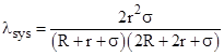
The total failure state 22 is just a place-holder, since a system leaves the population when it enters this state, and doesn’t return to the population until it is repaired or replaced by a system in state 00. Therefore, the rate ω is irrelevant to the hazard rate of the operational population. The system failure rate is the rate of entering state 22, which is

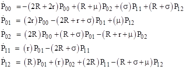
The system equations are

along with the conservation equation

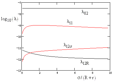
Setting the derivatives to zero and solving the resulting system of equations, we get P₀₂, P₁₁, and P₁₂, which we can substitute into equation (1) to give the system failure rate explicitly as a function of R, r, μ and σ.  The plot below shows the rates of the four ways of entering state 22 as a function of σ, given the parameters R = 10⁻⁵, r = (0.02)R, and μ = 1/150. The upper line represents the rate of entering state 22 from state 02, which is by far the most likely way of reaching state 22. The red lines represent the rates triggered by the occurrence of the external threat, and as can be seen, the maximum contribution occurs for σ near the square root of 2 times R + r.

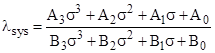
The overall system hazard rate is the sum of the four rates. Algebraically, the system hazard rate is

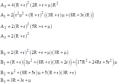
where the A_j and B_j coefficients are functions of R, r, and μ as shown below.

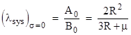
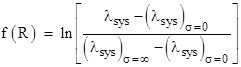
Now, if σ = 0, the system failure rate is

On the other hand, if σ approaches infinity, the system failure rate approaches

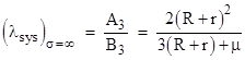
Notice that the last two expressions are identical, except that R is replaced with R + r. Depending on the values of the other parameters, the system failure rate may increase monotonically between these two levels, or it may pass through a maximum and drop back down, as illustrated in the two plots below.

In many applications the value of σ (the rate of encountering the external threat of sufficient severity to cause a unit failure) is unknown, so it is necessary to choose a conservative value. In the special case when μ goes to infinity (meaning that individual unit failures are repaired immediately) the above expression for the system failure rate reduces to

which is zero if σ is either zero or infinite. In this case we can differentiate with respect to σ and set the resulting expression equal to zero to find that the value of σ giving the maximum value of λ_sys is

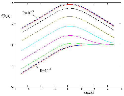
(This special case is discussed further in the note on Redundant Systems With A Common Threat.) Similarly if the repair time is non-zero, so μ is finite, we can determine a conservative value of σ by maximizing the full expression for the system hazard rate λ_sys. To characterize the general behavior of the system hazard rate function, suppose r = R/50, meaning that the rate of undetected failure of the threat protection features in any given unit is 2% of the detected failure rate of the unit, and choose units of time such that μ = 1 (so R and σ are now dimensionless multiples of μ). With these parameters fixed, a plot of the normalized logarithmic quantity

versus ln(σ/R) is shown below.

As in the case of instantaneous repairs, we find that the maximum (if it exists) occurs at approximately

and it asymptotically approaches this value as R becomes small. Even when f(R,σ) is monotonically increasing (which is the case for R greater than about (3)10⁻³), the curve flattens out at about this value of σ, so it is a reasonable approximation in all cases.

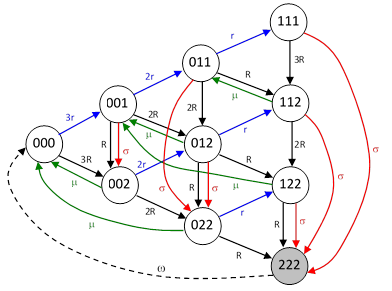
We can apply this same type of analysis to a 3-unit system, where each units can be either healthy, or with undetected failure of protection, or in a detected failure state. As before, we denote these by the indices 0, 1, and 2. The units are symmetrical, so the order doesn’t matter. Thus the subscript “012” (for example) signifies that one unit is fully healthy, one has failed protection, and one is in a detected inoperative state. The Markov model for this system is shown below.

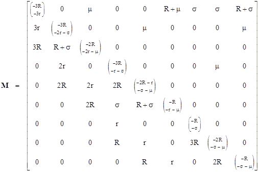
As explained for the 2-unit system, the total failure state (222) is just a place-holder, so there are only nine states of the system. For convenience we will number the states from 1 to 9 in the order 000, 001, 002, 011, 012, 022, 111, 112, 122.  By examining the model we can define the transition matrix M shown below.

In terms of this matrix the system equations are

where P is the column vector consisting of the probabilities of states 1 through 9. The eventual steady-state solution has dP/dt = 0 and therefore MP = 0, but since the rows of M sum to zero they are not independent. Replacing the first row of M with the condition that the sum of all the probabilities is unity, we have nine independent conditions, so we can solve for the probabilities. Letting A denote the modified version of M (i.e., with the first row replaced with 1’s), and letting C denote the column vector with C₁ = 1 and C_j = 0 for all j > 1, the steady state probabilities are given by

In terms of these probabilities, the total system failure rate can be read off the model diagram as

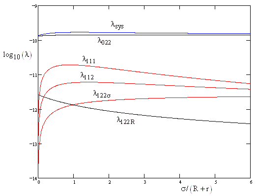
where we have reverted back to the original index notation for the various states. To illustrate, consider the case of a system comprised of three parallel units, each with a detected failure rate R = 10⁻⁵ per hour and undetected rate r = R/50 (i.e., 2%) of protection failure, and a repair rate μ = 1/150 hours. The five individual contributions to the overall system failure rate, along with the total rate, are plotted in the figure below (on a logarithmic scale).

Return to MathPages Main Menu