The Virial Theorem

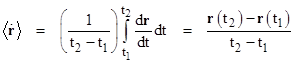
The asymptotic average of the derivative of a bounded function is zero. (Intuitively, if you drive around your parking lot for a long time, your average velocity approaches zero, because as time elapses your net distance traveled does not increase.) Formally this can be expressed by noting that, for any constant k and function r(t) bounded such that |r(t₂) – r(t₁)| < k for all t₁ and t₂, the average of the derivative of r over the range from t₁ to t₂ is

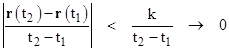
The magnitude of the numerator is bounded whereas the time interval t₂ – t₁ in the denominator can be increased without limit, so the asymptotic average of dr/dt as the time interval increases is zero, i.e.,

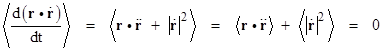
If both r and dr/dt are bounded functions of t, then so is their product, and it follows from the product rule that

Now, if r denotes the spatial position of a particle of mass m, then mr″ equals the net force F on the particle (by Newton’s second law), and m|r′|² is twice the kinetic energy T of the particle.  Thus if we multiply through the above equation by m we get

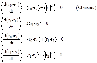
Consequently for a set of N particles with bounded positions r₁, r₂, … r_N, subject to the forces F₁, F₂, …, F_N, and with total kinetic energy T we have

This general proposition is known as Clausius’s virial theorem, and it has important applications in a variety of fields ranging from statistical mechanics to astrophysics.

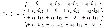
Suppose the forces on the particles are due entirely to mutual forces which the particles exert on each other. In such a case each F_i is the sum of the individual forces exerted on the ith particle by all the other particles. For example, with N = 4 particles, and letting f_ij denote the force exerted on the ith particle by the jth particle, we can write the virial theorem as

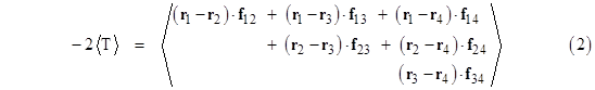
By Newton’s third law, we have f_ij = –f_ji, so the diagonally symmetrical terms can be matched in pairs, enabling us to re-write this in the form

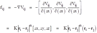
If we further stipulate that the force exerted on the ith particle by the jth particle points along the line through the two particles and varies in proportion to some power of the radial distance, i.e., if the force is of the form

for some integer n and constant K (recalling that we defined f_ij as the force on the ith particle, and the vector r_i – r_j points toward the ith particle), then the potential energy of this bond is

This can be confirmed by noting that

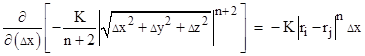
so the partial derivative of V_ij with respect to Δx is

and similarly for the partials with respect to Δy and Δz, from which we have the force

Therefore, since the potential energy of the bond between the ith and jth particles is equal to [–1/(n+2)](r_i – r_j)∙f_ij, the quantity on the right hand side of equation (2) is –(n+2) times the average of the total potential energy V of the system of particles. Thus equation (2) can be expressed as

The exponent of Δr in the expression for the potential is ν = n+2, so the above equation can also be written as

In the case of an inverse-square force, such as Newtonian gravity, we have n = –3 and ν = –1, so the virial theorem gives the simple relation

In words, this signifies that for any bound system of particles interacting by means of an inverse-square force, the average (negative) potential energy is twice the average kinetic energy.

Kepler’s third law is essentially a special case of the virial theorem for gravitationally bound systems consisting of a small particle in circular orbit around a large massive body. Noting the kinematic relation a = v2/r for circular motion, the combination of Newton’s second law and the law of gravitation gives

Multiplying through by r, we have

The left side is twice the kinetic energy and the right side is the negative of the potential energy, so this expresses the virial theorem for an inverse-square force, and if we multiply through by r/m we get Kepler’s third law

where ω = vr is the angular velocity of the orbiting particle. This relation can be used to determine the masses of astronomical bodies purely on the basis of the speed and radius of a satellite’s orbit.  For example, knowing the earth’s orbital velocity v and radius r, we can compute the mass of the Sun as M = v²r/G.

The same basic idea enables us to estimate the mass of a large agregate of bound objects, such as a galaxy of stars. By astronomical observations (involving measurements of optical intensity and doppler shift) we can count the approximate number, speed, separations, and masses of all the stars in the galaxy. From this information we can compute the overall kinetic energy T, and we can also determine the roughly static gravitational potential field produced by those stars, from which we get the overall potential energy V. Assuming the stars are bound by an inverse-square force (i.e., Newtonian gravity) we would expect to find 2<T> = –<V>, but in fact we typically find that 2<T> is at least an order of magnitude greater than –<V>. (The same is found for galaxy clusters.) Three possible ways of reconciling our analysis to the data present themselves.  First, we could infer that gravity is not an inverse-square force on the scale of galaxies. However, since the surface area of a sphere increases as the square of the distance, any deviation from the inverse square force law would imply a violation of Gauss’s theorem (unless we wish to postulate that space is correspondingly non-Euclidean on this scale). Also, for a general power law, we would be required to postulate a value of ν = –10 for a force proportional to the inverse-12th power, which hardly seems plausible.  Second, we might hypothesize that some other (i.e., non-gravitational) force becomes significant at great distances, but this is nearly the same as assuming a different form for the gravitational force at these distance. The third approach is to conclude that the galaxies contain at least ten times more matter than is visible to us in our astronomical surveys. This is the basis of the “missing mass” problem in astronomy, and it seems to be the most likely possibility, because there’s no reason to suppose most mass is radiating brightly enough to be visible.

For another example, consider a simple mass-spring system, for which the force on the mass m is directly proportional to the distance x from the origin. The equation of motion is

which has the homogeneous solution x(t) = Asin(ωt) where ω² = k/m. In this case the potential energy is (1/2)kx², so n = 2, and the virial theorem implies that <T> = <V>, which we can confirm by noting that the instantaneous kinetic and potential energies are

The long-term averages of cos(ωt)² and sin(ωt)² are equal, so if we substitute k/m for ω² into the expression for T(t) we find that the average kinetic energy does indeed equal the average potential energy.

Needless to say, Clausius’s virial theorem is just one of infinitely many propositions that follow from the fact that the average of the derivative of a bounded function is zero. Clausius’s theorem is based on the derivative of rr′, but we can just as well consider other functions, assuming r and all its derivatives are bounded. A few examples are listed below, using subscripts to denote derivatives with respect to t.

The last of these explains why there is an ambiguity in the question of whether radiation from a charged particle should be attributed to the second or the third derivative of the particle’s position (as discussed in Does AUniformly Accelerating Charge Radiate?).

It’s easy to see that the average of the dot product of any two consecutive derivatives is zero, as illustrated by the second identity above. More generally, we have

for any non-negative integers n and k. In other words, the average of the dot product of any two derivatives with orders differing by an odd number is zero. This is why the interesting identities involve only products of derivatives with orders differing by even numbers. We can also infer the following generalization of Clausius’s theorem

and even more generally

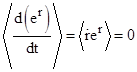
Many other identities follow in the same way. For example, if the scalar function r(t) is bounded then so is e^r, so we have

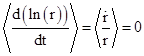
which is quite a bit stronger that just the fact that the average of dr/dt is zero. Likewise if r(t) is bounded away from zero then ln(r) is bounded, and we have

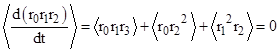
Another set of identities can be determined from triple products, such as

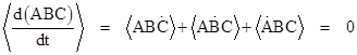
and more generally for any three bounded functions A(t), B(t) and C(t) we have

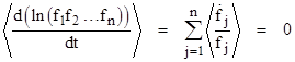
Extending this identity to the natural log of the product of n non-zero bounded functions f₁(t), f₂(t),…, f_n(t) gives

Return to MathPages Main Menu