Mnemonic Coins and Pattern Avoidance

One of the standard assumptions about tosses of a “fair coin” is that a coin has no memory, which is to say, the probability of any particular outcome on the next toss is independent of the outcomes of previous tosses. For example, if a coin has just come up heads ten times in a row, we might think it is almost certain to come up tails on the next toss, because it is “overdue” for tails, but this is not the case. The probability of heads is exactly 1/2 on the next toss, just as it was on each previous toss – assuming it is a standard fair coin.

However, we can also consider a coin with memory. Such a coin could still be “fair” in the sense that it does not inherently favor one outcome over another. For example, we could define a coin that has, on any given toss, a probability of 2/3 to come up the same as it did on the previous toss, and a probability of 1/3 to come up differently than the previous toss. This rule treats heads and tails equally, so it is nominally “fair”, and the asymptotic fractions of heads and tails are both 1/2, but there are local correlations between consecutive tosses. Even though the explicit memory of the coin extends back only one toss, the non-standard correlations are carried over an infinite number of tosses, albeit decreasing in significance exponentially. (Strictly speaking, such a coin would resemble a purely monochromatic wave in the sense that it could have no beginning.)

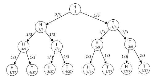
Suppose one of these mnemonic coins came up heads on the nth toss. The possible results on the subsequent sequence of tosses would be as shown below.

Thus the outcomes of the third toss following a head have the a priori probabilities

It’s easy to show that the probabilities of heads and tails on the kth toss following a head are

which implies that the difference between the a priori probabilities of heads and tails on the kth toss following a head is 1/3^k, so the overall probabilities converge on 1/2.

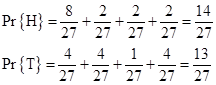
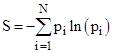
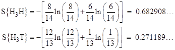
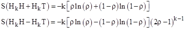
It’s interesting to observe that the probabilities are partitioned very differently into the 2^k−1 distinct paths that can be followed to reach each of the two outcomes. In the above example, the probabilities of the four individual paths leading to Heads are proportional to 8,2,2,2, whereas the probabilities of the paths leading to Tails are 4,4,1,4. Recall that the entropy of a macrostate possessing N possible microstates with conditional probabilities p₁, p₂,.., p_N is defined (with suitable units) as

where p₁ + p₂ + … + p_N = 1. By analogy, we can define macro-sequences based just on the beginning and ending states of a sequence, and we can define each possible path from the specified beginning to the specified ending state as a micro-sequence of the system, then the “entropies” of the two macro-sequences H₃H and H₃T are

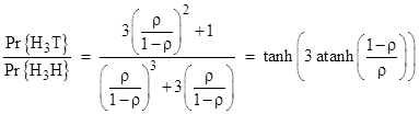
Thus the less probable macro-sequence H₃T has the higher entropy, which is somewhat counter-intuitive, but of course we’re taking liberties with the concept of entropy here. Partitioning a given probability in various ways doesn’t change the total probability. In the thermodynamic sense the entropy of a system refers to partitionings of the system’s energy, and the systems tends toward a macrostate that has the greatest number of representative microstates – assuming each microstate is equally likely. The direct analog to this, for coin tosses, would be to count the number of “ways” of length k from a Head to a Head, and compare this with the number of “ways” from a Head to a Tail. We must then decide what to call a distinct “way”. For example, we could limit our attention to just the number of reversals that a sequence cointains. On that basis there are just two distinct “ways” of going from Head to Head, namely, with zero reversals or with two reversals. These two ways have the conditional probabilities 8/14 and 6/14 respectively. Similarly there are just two ways of going from Head to Tail, namely, with one reversal or three reversals, and these have the probabilities 12/13 and 1/13. Thus the entropies for the two alternatives are

From this point of view the more probable outcome has the greater entropy, just the opposite of what we saw before. This shows an inherent ambiguity in the abstract concept of entropy, because every outcome can be considered as a representative of many different classes (macrostates), with differing entropies. The criteria for making the micro and macro classifications must be fully specified in order to give a rigorous definition of entropy. In the following discussion we will consider just the previous criteria, where the ordering of reversals (not just their number) is taken into account.

The conventional way of approaching a system of this kind is by means of a state vector and transition matrix. We have the two basis vectors

and the transition matrix

where ρ is the probability that the next outcome will be the same as the previous outcome. Given any state P[n] of the system, the state P[n+1] after the next toss is P[n+1] = MP[n], so the state after the kth toss is

To give explicit expressions for the components P₁[k] and P₂[k] of the state vector, we first determine the eigenvalues by solving the characteristic equation

This gives λ₁ = 1 and λ₂ = 2ρ−1. Each component of the state vector is of the form

for constants c₁ and c₂ determined by the initial conditions. Thus if P[0] = H we have

Unfortunately it isn’t immediately obvious from this approach how to determine the entropies of these macro-sequences, for which we need the probabilities of the individual micro-sequences. To find these, notice that, for k steps, all the paths with an even number of reversals give the same final result as the initial result, whereas all the paths with an odd number of reversals give opposite results. Also, the number of paths with k steps containing r reversals is the binomial coefficient C(k,r). Therefore, the probabilities are sums of alternate terms of the binomial expansion of [ρ + (1−ρ)]^k. For example, with k = 3 we have

In general this gives the probability of a macro-sequence as a sum of the probabilities of its micro-sequences

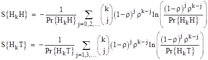
The entropies can then be expressed as

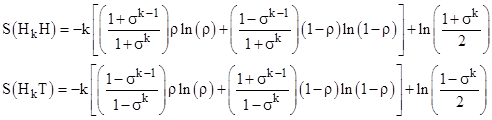
The substitution ρ = (1+σ)/2 helps to simplify these summations, leading to

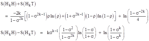
From this we get the sum and difference

The second equation shows that the difference with k = 1 is identically zero, regardless of the value of ρ. It should also be noted that the first of these equations is the sum of the entropies of the two macro-sequences, not the entropy of the union of those two sequences, and likewise the second equation is the difference between the entropies of the two macro-sequences, not the difference between the two components of the combined sequences. This is because entropy is based on the conditional probabilities, normalized so that the sum of the probabilities for the state in question is unity. If instead we combine both H_kH and H_kT into a single macro-sequence, then we normalize the probabilities over the entire set. This gives

The first of these shows that the total entropy increases directly in proportion to k, e.g., for ρ = 1/2 the total entropy for macro-sequences of length k is S_k = ln(2) k. The difference in entropy changes in proportion to k(2ρ−1)^k−1, so if ρ is greater then 1/2 (meaning “sameness of results from one toss to the next is preferred) this difference is monotonic increasing, whereas if ρ is less than 1/2 (meaning reversal is preferred) the difference alternates in sign.

Since the macro-sequence probabilities are alternating terms of a binomial expansion, their ratio can be expressed in terms of the hyperbolic tangent. For example, with k = 3 we have

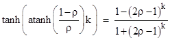
where we have made use of an identity discussed in Tangents, Exponentials, and π. In general we have the relation

which of course is just an expression of the trigonometric identity

The basic concept of a mnemonic coin, with the probabilities on kth toss determined by the outcome of the (k−1)th toss, can be extended in several ways. For example, we can just as well consider an n-sided die with probabilities defined as functions of the previous rolls. A six-sided die would have six “basis states” F₁, F₂, …, F₆, corresponding to the six faces of the die. Given any initial state P[0] = F_j, and a 6x6 transition matrix M, the probabilities on the kth roll are

Of course, just as in the case of the coin, this formula gives the a priori probabilities, without knowledge of the results of any rolls subsequent to P[0]. The above equation is linear and gives the dynamics of the system in terms of probabilities for each of the possible outcomes, rather than by predicting the actual results of the rolls. Thus the state vector evolves away from the initial basis vector P[0], and it not thereafter equal to any of the basis vectors for as long as it continues to be governed by that equation. If, however, an observation is made at some point, the die is found to be in one of the six basis states, so the state vector “collapses” onto one of those six observable states.

The six basis vectors corresponding to the six sides of the die are not the only possible set of basis vectors. In effect they define a certain measurement, namely, looking to see which face of the die is showing, and the observable result of such a measurement is one of the six faces. Those basis vectors are orthogonal unit vectors in a six-dimensional space, but we could rotate them to give a different set of basis vectors, and we could define a measurement for that basis such that when such a measurement is made, the state vector collapses onto one of those six basis vectors.

Another way of extending the original idea of a mnemonic coin is by making the probabilities on the next toss depend not just on the immediately preceding toss, but on several or all of the preceding tosses. We can never know the infinite past history of such a coin, so strictly speaking it would be totally unpredictable unless we place some restriction(s) on the possible dependencies. One natural rule that would render the system finitely predictable is given by assigning Heads to the binary number 1 and Tails to the binary number 0, and then defining the number C as the binary number whose digits correspond to the results of the previous tosses. The coefficient of 2^−j signifies the result of the jth prior toss. The most recent toss is encoded as the coefficient of 2⁻¹, and the toss before that is encoded as the coefficient of 2⁻², and so on. At any given stage the coin “remembers” this one real number, and we may specify that this number defines the probability of 0 on the next toss, and of course it’s complement defines the probability of 1 on the next toss. If there has been a series of five 1s in a row on the previous five tosses, then number C would be 0.111110…, which is very close to 1, so it is almost certain the next toss will give a 0. Conversely several 0s in a row would give progressively greater probability of a 1 on the next toss.

Even though it has infinite memory, such a coin is virtually a finite-state machine, because the digits become less significant at an exponential rate. The outcomes on tosses 30 steps ago have almost no influence (1/2³⁰) on the next outcome. A coin like this seems to be what many people intuitively imagine when they think about coin tossing, because it embodies the concept of “overdue” results, i.e., the longer we go without seeing a 1 (for example), the more likely we are to see a 1 on the next toss. However, it doesn’t entirely capture the intuitive sense of “saturation”, because if the coin has come up tails a million times in a row, and then comes up heads once, the value of C is 0.1000000…, so the probability of tails on the next toss is 1/2, even though we might be inclined to expect that we are still very “overdue” for heads. To remedy this we could weight the prior toss results more evenly, but we can never achieve a perfectly uniform distribution over the infinitely many tosses in the past (even if it were feasible for a finite coin to possess an infinite amount of memory).

Another respect in which such a coin does not embody common intuitions is that it doesn’t account for (and avoid) all possible “patterns”. If the previous tosses were alternately heads, tails, heads, tails, etc… we are likely to expect that this pattern should soon be broken, but a tendency to avoid runs of identical consecutive results also tends to favor consecutive alternating results. Of course, even if we devise a probability rule to avoid both runs of identical results and runs of alternating results, there are still other patterns that we will not be avoiding, and in fact that we will be favoring, simply due to avoiding other types of patterns. This highlights the well-known difficulty of producing high-quality pseudo-random sequences of numbers. The systematic avoidance of patterns is, in a sense, a self-contradictory task.

Return to MathPages Main Menu