Maxwell and Second-Degree Commutation

As discussed in another article, Maxwell’s equations can be expressed in the form

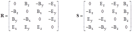
for ν = 1,2,3,4, where the super-scripted variables x¹,x²,x³,x⁴ represent the usual x,y,z,t inertial coordinates, τ is proper time along the path of the moving charge density, and the matrices R and S are

The two matrices R and S are related by the identities

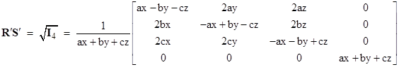
where I₄ is the 4x4 unit diagonal matrix. It’s worth noting that the quantities B² – E² and E∙B are the only two scalar invariants of the electromagnetic field. The first of the above identities implies that if we define

then we have

Thus the product of R′ and S′ is a square root of the identity matrix, even though it is not equal to the identity matrix. One way of expressing S′ in terms of R′ is

In the field of 4x4 matrices there are many “square roots of identity”. The particular one that is relevant here is the matrix

where the symbols a,b,c denote the components E_x,E_y,E_z, of the electric field, and the symbols x,y,z denote the components B_x,B_y,B_z of the magnetic field. The determinant of R′S′ is 1, the trace is 0, and the characteristic polynomial is

so the eigenvalues are ±1.

Lorentz’s force equation F = q(E + v x B) for a particle of constant rest mass m and charge q can be expressed properly in terms of R as

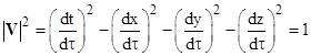
where V is the particle’s 4-velocity V = [dx/dτ, dy/dτ, dz/dτ, dt/dτ]^T. Since the magnetic force is always perpendicular to the velocity, it does not change the kinetic energy of the particle, so the entire contribution to the fourth component of the “force” vector (i.e., the change in energy with respect to time) is simply qE∙v.

In a region of space-time where the electric and magnetic fields are constant, the solution of equation (2) would be

but since R is actually a function of τ (meaning that the electric and magnetic fields vary along the worldline of the particle) we must split up each finite segment of the path into incremental parts over which R may be taken as constant, and then apply the above equation to each part, and then combine all these to give the result

Of course we also have the auxiliary equation

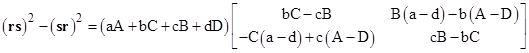
It’s interesting that although R and S don’t commute, they satisfy what could be called “second degree commutation”, i.e.,

If we consider two arbitrary 2x2 matrices

The second-degree commutator is

This matrix, which we will denote as [r,s]₂, is distinct from the commutator of the squares of r and s, and it vanishes if and only if

The left hand condition represents the vanishing of the first-degree commutator [r,s]₁, so the unique second-degree condition is the one on the right. If r is the transpose of s then [r,s]₂ vanishes but the leading factor is the sum of the squares of the components of r. On the other hand, if s is formed from r by transposing a and d, and negating b and c, then [r,s]₂ again vanishes but the leading factor is twice the determinant of r. Another way of writing the unique second-degree commutation condition is as the vanishing of the dot product [a,b,c,d] ∙ [A,C,B,D] = 0.

If we define the scalar product of two matrices as the sum of the products of their corresponding components, then this condition can be written as r ∙ s^T = 0. Thus if we map the 2x2 matrices to the four-dimensional vectors, then the matrices with which a given matrix commutes in the second degree are those whose vectors, after transposition of the B and C components, are perpendicular to the vector of the given matrix. This can be seen as an expression of the fact that two matrices must be independent (i.e., orthogonal, in this sense) if they are to commute at the second degree. Interestingly, for the 4x4 matrices R,S discussed previously, which commute in the second degree, we also have R ∙ S^T = 0.

Return to MathPages Main Menu