Reliability of Series-Parallel Systems

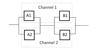
Consider a series-parallel system as shown schematically in the figure below.

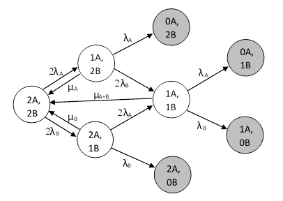
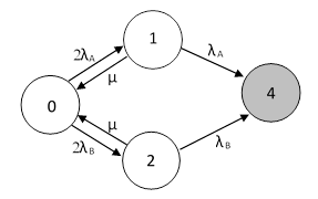
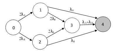
In order to remain operational, the system requires at least one of the modules A1 or A2 to be functioning, and at least one of the modules B1 or B2 to be functioning. Channels 1 and 2 are symmetrical. The Markov model for this system is shown below.

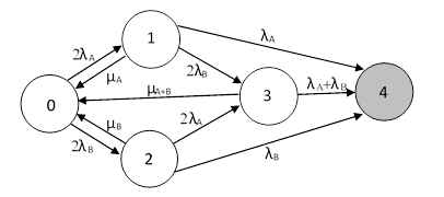
The notation in each state signifies how many of the A and B modules are operational. For example, “2A,2B” signifies that both of the A and both of the B modules are functioning. The shaded states are those that have lost both A modules or both B modules, so the system is inoperative. We can consolidate the inoperative states into a single state, and re-draw the model as shown below.

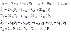
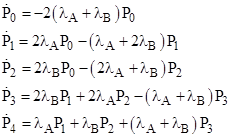
The equations of state are

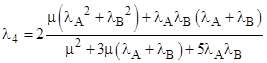
If we stipulate that the system will be repaired almost immediately if it enters State 3 (i.e., if State 3 is a “non-dispatchable” condition) and if we assume for simplicity that the repair rates for A and B faults are the same (i.e., μ_A = μ_B = μ), then the closed-loop steady-state hazard rate for State 4 is

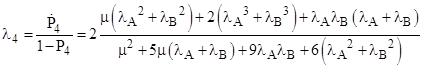
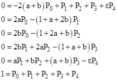
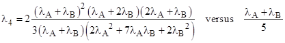
On the other hand, we might assume the repair rate from State 3 is the same as the repair rates from States 1 and 2. (We could also assume the repair rate from State 3 is some fixed multiple of the other repair rates, since the transitions are not really memoryless, but this is a separate issue.) Then, assuming this rate is non-zero, we can divide through the steady-state equations by μ and write the equations in terms of the dimensionless ratios a = λ_A/μ and b = λ_B/μ as follows

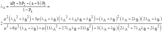
where e is an arbitrary closure rate. Solving this system (omitting the redundant penultimate equation) for the closed-loop steady-state hazard rate of State 4 gives

If the repair rate is sufficiently large compared with the failure rates, this approaches

Often in the analysis of parallel-series systems the dual-failure state is neglected. In other words, State 3 is omitted and the analysis is based on the simplified model shown below:

Solving for the closed-loop steady-state solution of this system gives

Again we find that if the repair rate is sufficiently large this approaches

which is the same as with the previous model. At the other extreme, i.e., with no repairs at all (μ = 0) the two models give

If λ_A = λ_B = λ then these results are

Not surprisingly, the simplified model gives a lower rate, because it excludes some of the paths for going from State 0 to State 4.

This illustrates the main limitation of Markov models, which is the difficulty of handling multi-level combinations of failures, even without repair transitions. This type of problem arises in the analysis of individual missions (such as individual flights of an airplane), during which no repairs are made, but multiple failures could occur (and the order of the faults is irrelevant). For this type of analysis, fault trees provide a much more efficient approach, because they make use of the Boolean representation of combinations of faults. For example, consider again the simple series-parallel system discussed above, but with no repair transitions. The Markov model for this system is shown below.

The equations of state are

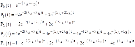
It is straight-forward but somewhat laborious to solve this system of five differential equations with the initial condition P₀(0) = 1 to give the time-dependent state probabilities

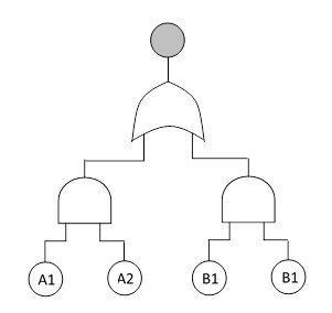
As an alternative approach to the same problem, consider the fault tree shown below for the same series-parallel system.

For independent events X,Y the probability of X and Y is P(X)P(Y), and the probability of X or Y is P(X) + P(Y) - P(X)P(Y), so the time-dependent probability of the top event (corresponding to State 4 of the Markov model) is trivially computed as

which of course is exactly the same as the result from the Markov model, but with much less labor. This is a fairly trivial combinatorial problem. Some systems involve highly complex logical combinations of failures, and the Markov approach quickly becomes impractical, whereas the fault tree method can handle them quite easily. The difficulty for fault trees arises when the basic events are not independent, in which case the simple probability formulas for “and” and “or” operations are not applicable, and it becomes necessary to analyze the problem algebraically in full generality. For large fault trees the number of Boolean terms to be evaluated can grow exponentially. This is a computationally intractable problem (it is known to be “NP complete”), so the best possible result is to find a means of rigorously proving robust upper and lower bounds on the probabilities. This can be accomplish using truncation with residuals.

Return to MathPages Main Menu