The Resultant and Bezout's Theorem

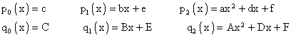
Suppose we wish to determine whether or not two given polynomials with complex coefficients have a common root. Given two first-degree polynomials a₀ + a₁x and b₀ + b₁x, we seek a single value of x such that

Solving each of these equations for x we get x = -a₀/a₁ and x = -b₀/b₁ respectively, so in order for both equations to be satisfied simultaneously we must have a₀/a₁ = b₀/b₁, which can also be written as a₀b₁ - a₁b₀ = 0. Formally we can regard this system as two linear equations in the two quantities x⁰ and x¹, and write them in matrix form as

Hence a non-trivial solution requires the vanishing of the determinant of the coefficient matrix, which again gives a₀b₁ - a₁b₀ = 0.

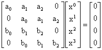
Now consider two polynomials of degree 2. In this case we seek a single value of x such that

for given complex coefficients a_j and b_j. As in the previous case we could solve each equation for x and equate the two resulting expressions, but it's more convenient to take the formal matrix approach. However, in this case we have two linear equations in the three quantities x⁰, x¹, and x², so the system appears to be under-specified. To eliminate x from these equations we can multiply through each equation by x, giving two more equations

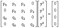
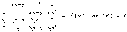
Together with the original two, we now have four linear equations in the four quantities x⁰, x¹, x², and x³, i.e., we have the system

Again, in order for the polynomials to have a common root, the determinant of the coefficient matrix must vanish, which in this case implies

Notice that the individual terms are of the same "degree" in the sense that the sum of subscripts of each term is equal to 4.

More generally, given any two polynomials f(x) and g(x) of degrees m and n with m ³ n, we initially have two linear equations in the m+1 quantities 1, x, x², ..., x^m. If n is less than m we can add m-n equations by multiplying g(x) by x¹, x^m, ..., x^m-n in turn, resulting in a system of 2+m-n equations in m+1 quantities. If n = 1 we can eliminate x from the system. If n is greater than 1 we need to augment the set of equations further by multiplying each one by k additional powers of x in turn. This results in 2+m-n+2k equations in m+1+k quantities x⁰, x¹,..., x^m+k. In order for the system to be solvable we must have 2+m-n+2k = m+1+k, and therefore k = n-1. Consequently we arrive at a system of m+n linear equations in m+n quantities. As an example, consider the pair of polynomials

Since these are of degree m=3 and n=2, we get the system of order 5 shown below.

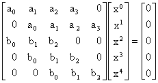
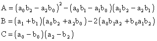
Again the vanishing of the determinant of the coefficient matrix is a necessary and sufficient condition in order for the two equations to have a common root. In this case the sum o the subscripts of each term in the expression for the determinant is. In general if each row of a matrix consists of a sequence of elements with arithmetically increasing powers of a unit, then the determinant is homogeneous, of degree equal to the sum of the degrees of the trace (main diagonal) elements. (Recall that the determinant of a square matrix of size N is defined as the sum of all products - with suitable signs - of N components chosen one from each column and row. Therefore one term is the product of the diagonal components, and every other term can be formed by row or column transpositions, each of which, under the stated conditions, preserves the degree of the trace product.) By construction, our diagonal consists of n copies of a₀ and m copies of b_n, so the degree of the determinant is the product mn.

The solution of systems of linear equations was apparently known in China, circa 200 AD, and the application of this method to eliminate the variable x from two polynomials was developed there in the 12th century. These techniques came into use by European mathematicians only around the 17th century, motivated by the identification of geometrical curves with algebraic equations. The study of curves and their points of intersection led naturally to the study of polynomials and their common roots. In order for an equation to represent a continuous locus of points (rather than just a finite number of discrete points) we need an equation of two variables. For example, straight lines are represented by the set of points with orthogonal coordinates x,y that satisfy a given algebraic equation of the form ax+by+c = 0 where a,b,c are constants. A different set of constants A,B,C would yield a different line, with coordinates satisfying the equation Ax+By+C = 0. Thus each curve corresponds to a polynomial.

The union of two curves obviously corresponds to the product of the two polynomials, because the union consists of the points x,y whose values cause either of the two polynomials to vanish. The intersection between two curves consists of the pairs x,y that that satisfy both of these equations. We might think this could be represented by the sum of the squares of the two polynomials, based on the idea that this sum vanishes if and only if both individual polynomials vanish. For example, given the straight lines corresponding to ax+by+c and Ax+By+C we could try to represent the intersection by the polynomial

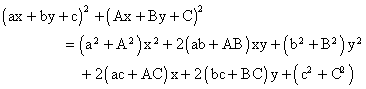
(Incidentally, the discriminant of this polynomial leads to the Fibonacci identity

signifying that the product of two sums of two squares is a sum of two squares.) Solving the sum of squares equation for y in terms of x gives the two roots

Thus there are infinitely many points on the complex plane with coordinates x,y such that the sum of squares of the two linear polynomials vanishes. Of course, if we stipulate real coordinates, the imaginary term must be set to zero, which singles out the specific point

So, if we restrict ourselves to points with real coordinates, the sum of squares can be used to represent the intersections of two curves, but this restriction cannot be conveniently encoded in an algebraic formalism, because polynomials generally have complex roots. We must solve for the complex roots of the polynomial given by the sum of squares, and then take the vanishing of the imaginary part as the condition identifying the intersection points. This becomes progressively more difficult for curves of higher degree.

For the intersections of two conics (i.e., plane curves of degree 2), the sum of squares would lead to an equation of degree 4, and the explicit expression for y in terms of x would have an imaginary part proportional to a 4th-degree polynomial in x. Due to the difficulty of algebraically solving 4th-degree polynomials (not the mention the impossibility for polynomials of higher degree), a more practical approach is to eliminate one of the two variables from the original two equations using the standard method of linear elimination described previously. To illustrate, consider a conic, i.e., a plane loci consisting of points with coordinates x,y such that

where a,b,...,f are constants. A different set of constants A,B,...,F yields a different conic curve, with coordinates satisfying the equation

To find the intersection of these two curves, we can re-write them in the form

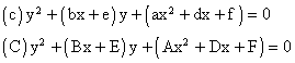
Treating these as two 2nd-degree polynomials in y, we can use the method described previously to find the necessary and sufficient condition for a single value of y to satisfy both equations. For convenience we define

Then as before we have the system of equations

Setting the determinant of the coefficient matrix to zero, we get

Substituting for the p and q functions gives a polynomial of degree four in the single variable x. This is called the resultant of the two original polynomials. The roots of this quartic give the x coordinates of the (in general) four points of intersection between the two conics. Naturally this includes complex points of intersection if there are any, and it counts repeated roots. Of course, this assumes the polynomials representing the two curves have no common factor, because if they share such a factor they obviously intersect at each of the infinitely many points of that common factor. Also, strictly speaking, we need to consider the "points at infinity" of the projective plane in order to claim that there are always exactly four points of intersection between two conics.

We saw previously that if m and n are the degrees of the coefficients of the two original polynomials, then the degree of the resultant is the product mn. Thus we can assert that, taking into account complex, repeated, and projective points, two algebraic plane curves of degrees m and n with no common factor intersect in exactly mn points. The first person to state this may have been Isaac Newton. In 1665 while a student at Cambridge he composed some notes on "the geometrical construction of equations", containing the comment

In 1720 Colin Maclaurin wrote a treatise on algebraic curves and asserted this same proposition, as did Euler and Gabriel Cramer in 1748, but none of them gave a valid general proof. Today the proposition is known as Bezout's Theorem, named after Etienne Bezout (1730-1783), who developed the theory of determinants and resultants. Bezout offered a proof of this theorem in 1779, but it did not correctly account for the multiplicities of intersection points in all cases. Apparently the general proposition was not fully established until Georges-Henri Halphen's proof, published in 1873. An elementary proof was also published by van der Waerden in 1930.

It's interesting that Gauss' celebrated first proof of the fundamental theorem of algebra in his doctoral dissertation (1799) invokes Bezout's Theorem, despite the fact that a satisfactory proof of this theorem itself relies on the fundamental theorem, which in turn relies on a rigorous treatment of continuity that was also unavailable to Gauss, so his 1799 proof of the fundamental theorem is nowadays considered somewhat lacking in rigor.

To formally account for the "points at infinity" we need to work in the projective plane. The usual construction of the projective plane is to replace each pair of coordinates x,y with the ratios x/z, y/z for some arbitrary z, so each point is represented by three coordinates x,y,z, with the understanding that only the ratios of these three components are significant. In other words, (x,y,z) is the same point as (lx,ly,lz) for any l. For any z not equal to zero this set of points maps to the points of the ordinary plane, but the points of the form x,y,0 represent points at infinity, one for each direction in the plane.

To illustrate, consider the intersection of the two lines 3x-2y+5 = 0 and 3x-2y+1 = 0. These two lines are parallel, and if we eliminate y we also eliminate x, and we arrive at the impossible condition 4 = 0, which signifies that these two lines have no point of intersection in the ordinary plane. However, if we replace x and y with x/z and y/z, and multiply through by z, the equations of the lines are 3x-2y+5z = 0 and 3x-2y+z = 0. These are homogeneous equations, and if we eliminate z we get the condition 2y = 3x, which implies z = 0. Hence the intersection between these two lines in the projective plane is the point (2l,3l,0). In contrast, if we eliminate z from the projective equations for two non-parallel lines 3x-2y+5z and 4x-7y+2z we get 14x = 31y, which implies z = (-13/31)x, so the point of intersection is (31l,14l,-13l), corresponding to the coordinates x = -31/13, y = -14/13 in the ordinary plane.

In general, given the polynomials for any two plane curves in the ordinary x,y plane, we can multiply through by powers of z to give the equivalent homogeneous equations in the projective coordinates x,y,z. We can then write the two equations as polynomials in z with coefficients that are polynomials in x and y. In other words, we have two equations of the form

The resultant of these two polynomials is, in general, a homogeneous polynomial of degree mn in x and y. Dividing through this equation by x^mn gives a polynomial in (y/x) of degree mn, so we have mn projective roots. Of course, we have divided out all common factors of x and y, so this may reduce the number of non-trivial roots.

It's worth noting that one or more of the coefficients of a polynomial can be zero, in which case we can get multiple roots. The most obvious example is for two homogeneous equations in the ordinary xy plane. To illustrate, consider the pair of equations

Since the degrees of these polynomials are 5 and 3, Bezout's Theorem implies that there are 15 points of intersection between them. However, for any non-zero x we can divide through these equations by x⁵ and x³ respectively to give two polynomials in (y/x). The loci representing the solutions of these equations consist of straight lines through the origin, where both equations are satisfied with x = y = 0. Thus all 15 points of intersection lie on the origin, so there is really just a single point of intersection with multiplicity 15. This shows the necessity of counting multiplicities in a suitable way if Bezout's Theorem is to be strictly true.

In the preceding discussion we relied on the algebraic degree of the resultant of the two given equations to tell us the number of intersection points of the corresponding plane curves (making use of the fundamental theorem of algebra). For a more visual and geometrical appreciation of Bezout's Theorem (given the fundamental theorem and the continuity of the roots of a polynomial under continuous changes in the coefficients), suppose the equations for two plane curves f(x,y) = 0 and g(x,y) = 0 of degree m and n respectively both have purely real roots when solved for x in terms of any real y, and vice versa. If this were the case, we could plot the m values of y such that f(x,y) = 0 as a function of x, and we could plot the n values of x such that g(x,y) = 0 as a function of y. The result would be as illustrated below for m=3 and n=2.

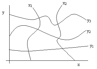
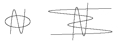
The m functions y₁, ..., y_m representing y at x such that f(x,y)=0 clearly (given the continuity of the root loci) intersect with the n functions x₁, ..., x_n representing x at y such that g(x,y)=0 in exactly mn points, counting multiplicities. Of course, this is too simplistic, because in general the "f" root values of y at a given real x can be complex, as can the "g" root values of x at a given real y. Therefore we cannot generally represent these root loci on a simple two-dimensional plane. Nevertheless, this shows intuitively that two equations - at least those whose roots are purely real in the range of overlap and of suitable degrees in x and y - ought to satisfy Bezout's Theorem. Indeed this is literally the case, as illustrated in the figures below. The left hand figure shows the six points of intersection of a conic with a cubic, and the right hand figure shows the fifteen points of intersection of a cubic and a quintic.

Can we extend this intuitive approach to cover cases when the intersections are complex? For any complex number x, and assuming f(x,y) is of degree m in y, we can determine the m complex values of y such that f(x,y) = 0, and if we focus on just the kth continuous root surface, each value of x maps to a unique value of y, which we denote as y = F_k(x). Likewise, assuming g is of degree n in x, we will let x = G_j(y) denote the mapping from any given complex number y to the complex number x such that g(x,y) = 0 for the jth continuous root surface of g. Then we have the composite function x' = G_j(F_k(x)). This mapping is reversible in the sense that for any given x' we can determine the corresponding value of x (for the jth and kth root surfaces). We need to show that this composite mapping from x to x' has a fixed point. It's easy to see that f and g can have no more than mn points of intersection, so if we can show that each of the pairs of root surfaces corresponds to at least one intersection point, we can conclude that each such pair contributes exactly one intersection point.

To show that the mapping between x and x' has a fixed point, we can project the complex plane onto a finite surface such as a hemisphere as shown below.

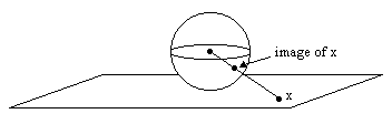
Now we can project the hemisphere continuously onto a finite square surface, on which we have the (projection of) a continuous bijective mapping between x and x'. According to Brouwer's fixed point theorem such a mapping possesses at least one fixed point.

In this argument we assumed that f(x,y) is of degree m in y, and that g(x,y) is of degree n in x. Naturally the same argument works if we replace x with y, but suppose neither of these is the case. For example, consider the two equations

Each of these equations is of degree 2, so according to Bezout's Theorem there are four points of intersection, but both equations are only of degree 1 in y, and if we eliminate y we get a quadratic in x

Likewise if we eliminate x from the two original equations we get a quadratic in y. Thus it would seem that there are only two points of intersection, whose x coordinates are given by the roots of this quadratic. However, in the projective plane the two equations are

and we can eliminate z by means of the resultant

where

If x is not zero we can divide through by x² and solve the resulting quadratic in y/x to give the two finite intersection points corresponding to the ones noted above. On the other hand, we now have two additional (duplicate) intersection points at infinity, corresponding to the two roots of x² = 0. With x = 0 the original equations are satisfied if and only if z = 0 for any arbitrary y, so we have a point at infinity (0,y,0) with multiplicity of 2.

Return to Mathpages Main Menu