The Hydrogen Atom

In 1885 a Swiss secondary school teacher named Johann Jacob Balmer published a short note (entitled “Note on the Spectral Lines of Hydrogen”, Annalen der Physik und Chemie 25, 80-5) in which he described an empirical formula for the four most prominent wavelengths of light emitted by hydrogen gas. These wavelengths had been measured with great precision by Vogel and Huggins, giving the four values 6562.10, 4860.74, 4340.10, and 4101.20 Angstroms (10^-10 m).  Balmer's note does not make clear whether he was also aware of the measured series limit, λ_∞ = 3645.6 A, or whether he deduced this himself.  In any case, one can find by numerical experimentation that the four characteristic wavelengths are closely proportional to the following products of small primes

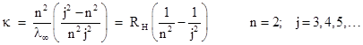
Three of these are divisible by 2³, three are divisible by 5, three are divisible by 7, and two are divisible by 3³.  Thus we can easily express these numbers as simple fractional multiples of 840 = 2³×3×5×7, which corresponds to the series limit λ_∞ = 3645.6 A.  It may have been just this kind of numerical experimentation that led Balmer to recognize that the four prominent wavelengths are given very closely by (9/5)λ_∞, (16/12)λ_∞, (25/21)λ_∞, and (36/32)λ_∞.  He also noticed that the numerators of the coefficients are consecutive squares, and each denominator is 4 less than the numerator. He speculated that the pattern would continue up to the series limit, which is indeed the case. In terms of the wave number κ (=1/λ), Balmer's formula can be written as

where R = n²/λ_∞ with n = 2.  The parameter R_H is now called Rydberg's constant for hydrogen, and the best empirical value is 10967757.6 m^–1.  As Balmer also speculated, if we take different values of n we get different series of spectral lines. The series with n = 1, 2, 3, 4, and 5 are now known as the Lyman, Balmer, Paschen, Brackett, and Pfund series, respectively, which characteristic the spectral lines of the hydrogen atom.  (The Balmer series was observed first because its frequencies are in the visible and near ultra-violet range.)  This is an outstanding example of a successful empirical fit (like Bode's Law in astronomy) for a class of physical phenomena that was not based on any underlying physical model or theory, i.e., no reason was known for why wavelengths of light emitted from a hydrogen atom should exhibit this pattern.

In classical terms a hydrogen atom consists of a proton and an electron bound together by their mutual electrical attraction.  To keep them from collapsing together, we might imagine that the electron is revolving in “orbit” around the proton, similar to a planet revolving around the Sun, with the centrifugual force balancing the electrical attraction.  However, this model is not satisfactory, because the electron would be continuously accelerating, and according to classical theory an accelerating charge radiates energy in the form of electro-magnetic waves. As a result, the orbiting electron would very quickly radiate away all of its kinetic energy and spiral into the proton. Thus the existence of stable atoms was inexplicable in the context of classical physics, as was the characteristic set of discrete energy levels of atoms.

By the early 1900's it had become clear that classical electrodynamics was inadequate to account for the behavior of either the electromagnetic field or of elementary particles.  In 1900 Max Planck had shown in his study of black-body radiation that it is necessary to quantize the energy of electromagnetism in order to avoid the "untra-violet catastrophe", and he introduced the fundamental constant h.  In 1905 Einstein made the even more radical proposal that in some respects electromagnetic wave energy propagates as if it consists of small packets (photons) with many of the characteristics of particles, each photon having an energy E related to the wave frequency ν by E = hν.

In 1913 Niels Bohr developed a new representation of the hydrogen atom by combining classical ideas with a few additional postulates that were suggested by the nascent quantum concepts of Planck and Einstein. First, he assumed that the angular momentum of an electron in orbit around the nucleus must be an integer multiple of  (Planck's constant h divided by 2π). It follows that only a certain set of discrete energy levels may occur. Second, he assumed that an electron radiates energy only when it makes a transition from one stable orbit to another of lower energy. If DE is the difference in energy levels, then he assumed that the transition resulted in the emission of a photon with this amount of energy, and hence with the frequency ν = ΔE/h in accord with Einstein's postulate. Armed with these postulates, Bohr reasoned that an electron of mass m orbiting a proton (of much greater mass) at radius r would satisfy the classical force balance

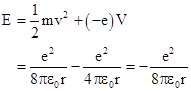
and the total energy (kinetic plus potential) has the classical value

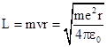
Likewise the angular momentum has the classical value

Bohr then imposed his quantization assumption, asserting that L must be an integer multiple of .  Setting L = n and solving the above equation for r, we get

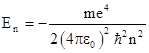
Substituting into the expression for the energy E gives the corresponding quantized energy levels of the hydrogen atom

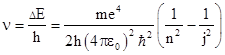
This provides a nice rationale for Balmer's empirical formula, because it implies that the frequency of the emitted light when an electron makes a transition from the jth to the nth energy level is

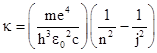
Since λν = c we have κ = ν/c and therefore

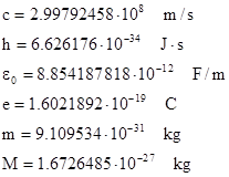
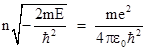
Actually, to be more accurate, the mass m in this expression should be replaced with the "reduced mass" mM/(m+M) where M is the mass of the proton (or, more generally, the nucleus), just as in classical orbital mechanics.  Then the coefficient in the above expression is identified with Rydberg's constant R_H for the hydrogen atom, and using the values of the fundamental constants

we can compute

This is in remarkable agreement with the measured value of 10967757.6 ± 1.2 m^–1 from spectroscopic data.  Nevertheless, Bohr's model of the atom is not completely satisfactory, partly because of the ad hoc nature of its premises, and also because it's representation of electrons as tiny particles with definite trajectories is not viable in a wider context. 

A somewhat plausible justification for Bohr's quantization postulate came in 1924 when Louis de Broglie developed the idea that particles of matter on the smallest scale exhibit wave-like properties, complementing Einstein's suggestion that electro-magnetic waves exhibit particle-like properties. The de Broglie wavelength for the matter wave corresponding to a particle with momentum p is λ = h/p, and if we stipulate that the circumference 2πr of a circular orbit of radius r must be an integer multiple of the wavelength, we have 2πr/λ = 2πrp/h = n for some positive integer n. Since the angular momentum is L = pr, this immediately gives Bohr's quantization postulate L = n. This "orbital wave quantization" is illustrated for n = 1 through 5 in the figures below.

However, despite the plausibility of this approach, Bohr's model of the hydrogen atom, even with de Broglie's justification and with subsequent refinements by Sommerfeld, is now considered obsolete, having been superceded by a more thorough-going wave mechanics developed by Erwin Schrodinger in 1925. (This new theory was subsequently shown to be essentially identical to the "matrix mechanics" already developed by Werner Heisenberg in 1924.)

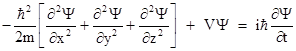
Schrodinger's wave mechanics postulates that a particle is characterized by a complex-valued wave function Ψ(x,y,z,t) whose squared norm at any point equals the probability density for the particle to be found at that point.  (The probability interpretation of Schrodinger's wave function was first proposed by Max Born.)  In addition, Schrodinger postulated that, in a region where there is a potential field V(x,y,z,t), the wave function Ψ of a particle is governed by the equation

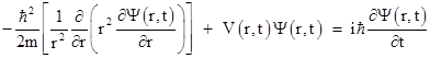
It's possible to give a plausibility argument for this equation, but here we will just take it as given. Expressing the spatial Laplacian (the quantity in the square brackets) in terms of polar coordinates, and considering just the radial part, this equation is

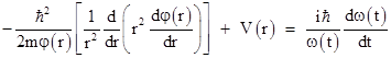
Furthermore, if the potential field V does not change with time, we can separate the variables by expressing Ψ(r,t) as a product of a spatial part and a temporal part, i.e., we have functions φ(r) and ω(t) such that Ψ(r,t) = φ(r)ω(t).  Substituting into the above equation and dividing through by Ψ(r,t) gives

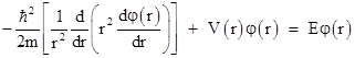
Since r and t are independent, the left and right hand sides of this equation must both equal a constant, which we will call E, so the time-independent radial Schrodinger equation in this simple case is

Now, as mentioned previously, for the region around a charged proton the potential energy due to the Coulomb force is given by

Inserting this into the Schrodinger equation, evaluating the nested derivatives, and re-arranging terms, we get

For sufficiently large values of r the terms with r in the denominator will be negligible, so the equation will reduce to

which has the solution

To exploit this asymptotic result, and without loss of generality, we can consider a general solution of the form φ(r) = F(r)e^–Cr.  Substituting into the Schrodinger equation, evaluating the derivatives, and dividing through by e^–Cr, we get

where

If the function F(r) is analytic it can be represented by a power series, i.e., it can be expressed in the form

Substituting into the equation for F, collecting terms by powers of r, and setting the coefficients of these terms to zero, we arrive at the conditions

for k = 1, 2, ...  For sufficiently large k these expressions approach f_k = [2C/(k+1)]f_k–1, which is the series for e^2Cr, and hence F(r)e^–Cr goes to e^Cr, which increases to infinity as r increases. Therefore, in order to give a solution that goes to zero as r goes to infinity, we must impose the requirement that the series for F(r) terminates after a finite number of terms. This occurs if and only if nC = B for some positive integer n. Hence the necessary and sufficient condition for the solution to approach zero as r increases is

Squaring both sides and solving for E gives the allowable energy levels

which is identical to the discrete energy levels of Bohr's model discussed previously.  It’s worth noting that the quantization of energy levels here is not the result of quantized angular momentum or orbital standing-waves. It arises from an analysis of the purely radial component of the Schrodinger wave equation of the ground state, which is spherically symmetrical and has an angular quantum number of zero.

Superficially it isn't obvious that the "realistic solutions" of (1) must be quantized, so it's worthwhile to examine the solution technique more closely to understand clearly how the quantization arises. First, notice that if we had tried to find a series solution of (1) directly by inserting a series φ(r) = φ₀ + φ₁ r + φ₂ r² + ... we would have arrived at a set of conditions involving three consecutive coefficients. This can be seen by inspection, because when we carry out the differentiations and collect the coefficients of r^k, any term of the original differential equation of the form r^s d^qφ/dr^q contributes a quantity involving φ_k+q-s.  Hence the four terms of (1) contribute quantities involving φ_k+2, φ_k+2, φ_k+1, and φ_k respectively.  In contrast, the four terms of (2) contribute quantities involving f_k+2, f_k+2, f_k+1, and f_k+1 respectively, so the power series conditions enable us to determine each f_k+2 as a multiple of f_k+1. We originally motivated the solution form F(r)e^–cr based on the asymptotic solution for large r, but we could also have justified it based on the fact that this transformation leads to a differential equation whose power series solution is subjected to conditions on just two consecutive coefficients. The fact that such a transformation exists is crucial for the quantization.

This leads us to consider the general conditions in which such a transformation exists.  Suppose we have a second-order differential equation of the form

where α, β, and g are rational functions of x.  Since we can multiply through by arbitrary polynomials in x, we can assume without loss of generality that α, β, g are polynomials in x.  If we postulate a solution of the form y(x) = f(x)e^g(x) and substitute into this equation, we get

In order for the series solution for f(x) to have conditions on just the sets of two consecutive coefficients, there must be an integer d such that the coefficient of f″ contains only terms in x^d+1 and x^d+2, and the coefficient of f′ contains only terms in x^d and x^d+1, and the coefficient of f contains only terms in x^d.  We seek a function g(x) such that these conditions are satisfied. In the case of equation (1) we have (after multiplying through by r) an equation of the form (5) with α(x) = x, β(x) = 2, and γ(x) = 2B – C²x where B and C are the constants defined previously. Therefore, from the condition on α, we see that d is either 0 or 1, so we need a function g(x) such that 2xg′ + 2 involves only terms in x⁰ and x¹, or only terms in x¹ and x².  Since it certainly involves a term in x⁰, the remaining term must be in x¹, so g′(x) must be a constant. Also, the coefficient of f must be in x⁰ (i.e., a constant), so we have x(g')² + 2g′ + 2B – C²x = K.  Therefore we must have (g′)² = (C)², which leads to the transformation y(x) = f(x)e^–Cx as expected.

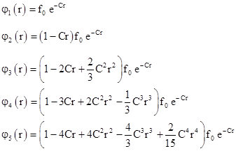
The superiority of the wave mechanical model of the hydrogen atom over Bohr's model is immense, because it not only duplicates and (in a sense) "explains" the quantized energy levels, it actually gives the complete probability density functions for the various possible stationary states. Using the recursive formula (3) we can evaluate the coefficients of the polynomial F(r) for each value of the quantum number n. Combining these polynomials with the exponential parts, we have the wave functions of the first few states

Recall that B = nC and B is composed entirely of fundamental constants, independent of n, and it has units of inverse length.  Letting a₀ denote the length 1/B = 1/(nC), and using m instead of the more accurate reduced mass, we have

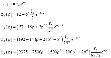
and we can substitute 1/(na₀) for C in the preceding wave functions and clear fractions.  In terms of the normalized radius parameter ρ = r/a₀ the wave functions are

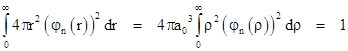
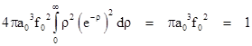
Each of these wave functions includes a constant factor f₀.  To determine the value of this factor, recall that the squared norm of the wave function is the probability density, and so the integral of this quantity over all of space must equal 1.  The volume of an incremental spherical shell of radius r and thickness dr is 4πr²dr so the probability integral is

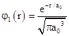
For example, to find the constant factor f₀ for the case n = 1 we insert the wave function into this equation and evaluate the integral to give

Therefore we have f₀ = (πa₀³)^–1/2, and the complete wave function for the ground state of the hydrogen atom is

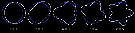
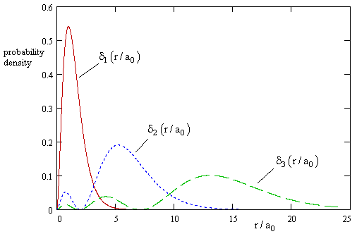
Of course, in accord with our choice of nomalizing factors, the probability density for finding the electron in an incremental shell of radius r is δ_n(r) = 4πr²φ_n(r)².  This is plotted in the figure below for the first few values of n.

Throughout this discussion we've ignored the angular components of the electron's wave function, effectively assuming that it has zero angular momentum, so the only non-zero quantum number was the radial one. This was all based on taking just the radial part of the Laplacian in the Schrodinger equation. If we had taken the angular parts we would have found that those too are associated with quantum numbers 0,1,2,..., and they contribute to the overall orbital wave function. However, the essential features of Schrodinger's approach to the hydrogen atom are already apparent in the purely radial part.

Return to MathPages Main Menu