Discrete Fourier Transforms

Fourier transforms have many important applications in all branches of pure and applied mathematics. Given an arbitrary function f(t), the basic idea is to decompose that function (over some finite interval) optimally into a sum of pure sine waves, and to find the frequencies, amplitudes, and phases of those waves.

Recall that the quantity Ae^θi can be regarded as a vector on the complex plane, with length A and directed at an angle θ up from the positive real axis. The real and imaginary parts of this quantity are Acos(θ) and Asin(θ) respectively. Multiplying any complex number by Ae^θi has the effect of scaling the magnitude of that number by A and "rotating" it in the complex plane through the angle θ.

Suppose we're given the sequence of values taken on by the function f(t) for t = 0, 1, 2, …, n–1. (We will refer to the independent variable "t" as the time, although it not literally be time.) It is most convenient to fit these points to a sum of exponentials

where θ = (2π/n). (We've applied the factor 1/√n because it makes the inverse transform work out nicely, as shown below.) We have n data points and n unknown coefficients, so we can solve for the coefficients to give an exact fit of our data points. Of course, this will give us a complex function of t, but the values will be purely real at t = 0, 1, 2, …, n-1, so the imaginary parts vanish at these points, which implies that if we simply omit the imaginary parts altogether we are left with a real function f(t) that passes through each of the original data points and consists of a sum of n cosine terms, each with its own amplitude, frequency, and phase.

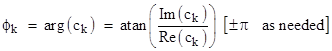
The coefficients c_j will generally be complex, which means they can be written in the form c_j = C_j exp(ϕ_j i) for some angle ϕ_j. Thus the entire jth term in the fitted expression for f(t) is C_j exp((jθt + ϕ_j)i), so ϕ_j represents the phase angle of this term. Omitting the imaginary part, the term becomes simply C_j cos(jθt + ϕ_j).

The sequence of coefficients c_j represents the Fourier transform of the time sequence f(t). The jth term corresponds to the frequency ω = jθ = j(2π/n) rad/sec (assuming the units of t are seconds). Thus our frequencies come in integer multiples of 2π/n, so the more often we sample, the better resolution of frequencies we will achieve.

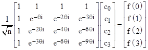
The straight-forward way of computing the coefficients c_j is by simply solving the system of simultaneous equations for the n data points. To illustrate, if we had just four data points, f(0), f(1), f(2), and f(3), we would solve this system of equations

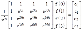
The inverse of the square matrix is given by simply negating each of the exponential arguments, and then multiplying the entire array by 1/n, as can be verified from the fact that the element in the jth row of the kth column of that matrix times its inverse is the sum

which equals n when j = k, and otherwise equals 0. Therefore, the inverse of the above matrix equation is

The sign in the exponentials just determines the direction of rotation of these periodic terms, so we see that the sequences f(t) and c_j are essentially duals of each other, meaning that each is the Fourier transform of the other. (It should be clear now why we divided by √n earlier, to make these transforms formally identical, up to the direction of rotation.) Let's call the square matrix multiplied by 1/√n in this equation E. Then the elements of the E array can be specified simply as

So, given the sequence of values f(t) as a column vector f we can compute the Fourier transform c(ω), which is column vector of n elements, by the equation

Obviously the inverse transform is simply f = E^–1c. The values of c represent the (complex) amplitudes of a set of n cosine functions with the frequencies

radians per [unit of t]. The power spectral density of the signal f(t) at a particular frequency is simply the squared amplitude at that frequency. In other words, the power spectrum can be represented as a column vector with the values

Notice that this covers the power of the signal over (1/n)th of the total frequency range. If we want to represent a smaller or larger band of frequencies, we would scale the amplitude accordingly.

The phase spectrum is similar to the power spectrum, except that it represents the phase angle corresponding to a given frequency. Thus is can be expressed as the column vector

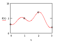
As an example, suppose we are given the sequence of values

Multiplying the column vector of these values by the 4th-order E matrix gives the Fourier transform

for w = 0, π/2, π, and 3π/2 radians/sec. The power spectrum is

at the frequencies 0, π/2, π, and 3π/2 radians/sec, so the predominant component is the DC signal. The amplitudes and phases of the four components are

Therefore, we have fit the function f(t) to the continuous function

where θ = π/2. A plot of this function is shown below:

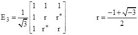
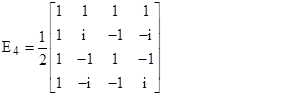
Incidentally, the E matrices for n = 2, 3, 4 are as shown below

This shows that the familiar reciprocal transform

is a primitive example of a Fourier transform. These simple discrete transforms occur quite often in quantum mechanics and the theory of relativity.

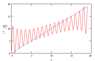
Another interesting aspect of the continuous representations given by the Fourier series for a linear sequence of discrete data points is illustrated by the case f(t) = t for t = 0, 1, …, 19. This is just a simple ramp function, but the 20th order discrete transform interprets it as an oscillating function as shown below:

This "smudging" of a linear ramp of data points is quite general, and applies to any number of data points, provided we perform an nth order Fourier transform on n points. However, it's worth noting that we don't need to use an nth order Fourier transform with n data points. Given a time sequence with many thousands of data points (say) we can apply multiple linear regression to fit a Fourier transform of any order less than or equal to the number of samples. (See the note on Multiple Linear Regression for details.)

Continuous Fourier transforms are essentially the same as the discrete transforms described above, except that we are given a continuous function f(t) instead of a finite set of discrete samples, and we replace the summations with integrations.

Return to MathPages Main Menu