Loxodromic Aliasing

If the ‘position’ of a system within the state space changes continuously, the path (though not the rate) of the system can be directly deduced from the locus of points it has occupied (up to direction), assuming the system never exactly backtracks. However, if a system changes it's position within the state space in discrete jumps, we can't unambiguously determine the path of the system merely from the locus of points it has occupied, because we don't know the sequence in which those points were occupied. In such circumstances, when describing the appearance of a sequence of states it may be necessary to account for aliasing.

An interesting example of this arises when we examine the apparent positions of distant stars to an observer who is subjected to a sequence of discrete Lorentz transformations. As Penrose pointed out, the angles of light rays through a given point in spacetime have a natural correspondence with the points of the Riemann sphere, and if we associate each of those points via stereographic projection with a point in the extended complex plane, the effect of any given (proper) Lorentz transformation on the ray angles in spacetime corresponds precisely to the effect on the complex plane of a certain linear fractional transformation w → (aw+b)/(cw+d) where a,b,c,d are complex numbers, normalized so that ad − bc = 1. Conversely, every LFT corresponds to a proper Lorentz transformation.

Now, suppose our observer is subjected to the Lorentz transformation corresponding to the LFT

where q equals, say, 1/100. We can normalize the coefficients if we like, to make ad − bc = 1.  The squared trace is obviously complex, so this is a loxodromic LFT. If we ask the observer to mark on a globe the apparent position of a particular star after each iteration of this function, what would we expect to see when he shows us the globe with all the markings?

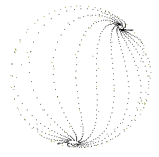
Naturally since the transformation is loxodromic, but just barely, we expect that if our observer tracked a star that began near the repelling fixed point he would have a single sequence of marks spiraling outward from that point and then ultimately spiraling inwards on the attracting fixed point. This is, in fact, what would appear to our eyes, but whether we would perceive it that way (at first) is questionable.  Here's a picture of the markings we would find on the globe:

At first glance this looks quite different from what we expected. Instead of a single spiraling path from one fixed point to the other, we find 13 distinct curvy paths! What has happened? If we ask our observer why he tracked 13 stars instead of just one as we had agreed, he will explain that he tracked only one star, and it did indeed spiral loxodromically (and monotonically) from one fixed point to the other. The explanation for the appearance of 13 curvy paths is simple aliasing, i.e., we are incorrectly inferring the path between the points, and in this case we are being strongly encouraged to do so by the arrangement of the points, each of which is in much closer spatial proximity to the point 13 steps ahead in the sequence than to either of its immediate neighbors in the sequence.

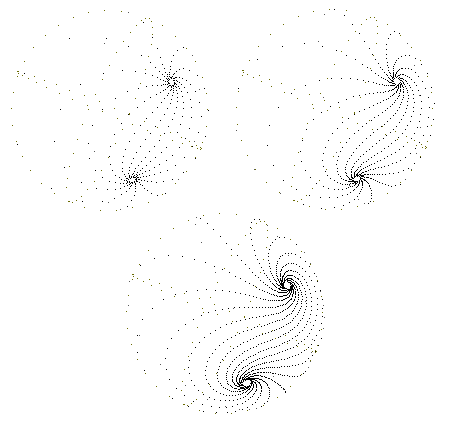
For another illustration, here are three "marked globes" for the transformation

with q = 0.02, 0.01, and 0.005, respectively.

Again we see (or seem to see) 13 curvy paths, and they actually approach being contiguous paths as q becomes smaller.

One question that might occur to us is "why 13"? It's worth noting that the sequence of loxodromic points almost gives just 7 curvy paths, because the cycle of pseudo-paths around one loop of the spiral is

This pattern, and in general the tendency for aliasing at various frequencies, is determined by how close the LFT is to being periodic with various periods.  It's easy to see that the LFT (aw+b)/cw+d) is cyclical with fundamental period m if and only if the squared trace equals  4cos(kπi/m)² for some integer k coprime to m. Since the squared trace also uniquely determines conjugacy, it follows that the number of distinct cyclical LFTs (up to conjugacy) with period m is ϕ(m) where ϕ is Euler's totient function.

In any case, we know the LFT (w+1)/(−w+1) is cyclical with period 4, so we would expect that if we make this loxodromic by inserting small imaginary components qi to each coefficient, we should see 4 distinct apparent "paths" connecting the two fixed points, which is indeed the case.

For those who like to speculate about the possibility of some kind of discretization of spacetime that nevertheless preserves Lorentz invariance, it might be interesting to consider whether the there is a special physical significance for the "cyclical" discrete Lorentz transformations.  Also, I think the general topic of aliasing is quite interesting. Of course, aliasing has well-known practical implications for things like signal processing and controls theory, but it's also interesting to consider how, in physics, identity is established between discrete appearances of ostensibly the same object at different times, and how we agree upon the "correct" sequence of events on the basis of necessarily incomplete information about our surroundings.

It seems that linear fractional transformations occur just about everywhere. For one example, see the article on Compressor Stalls and Mobius Transformations, which describes how stall cells migrate around the face of an axial compressor in a pattern corresponding to the action of a Mobius transformation on the complex plane. Also, for more on cyclical LFTs and the general closed-form expression for the nth composition of an arbitrary LFT, see Linear Fractional Transformations.

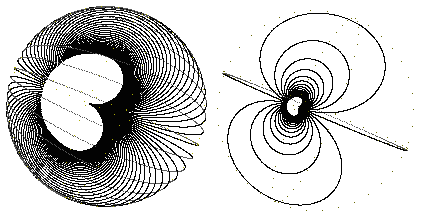
By the way, here are two images showing the effect of repeated applications of the Lorentz transformation corresponding to the parabolic LFT w → w + 0.01. The figure on the left shows the paths of points that begin on a semi-circle of radius 0.3 on the emitting side of the fixed point. The figure on the left shows the paths of points that begin on a semi-circle of radius 0.1, to show more detail of the short range "flux".

It may be worth mentioning that this progressive transformation of the celestial sphere can always be decomposed into a pure boost and a pure rotation. In other words, a second observer could travel along with the first, always exactly matching his velocity, but orienting his field of view always in the direction of the current boost relative to the initial frame, and this second observer will always see a simple contraction of the stars in front of him, i.e., an anti-podal repulsion from the point directly behind and attraction toward the point directly ahead. In a physical sense this axis is probably the most natural and significant in this context, since it is the "eigenvector" of the celestial transformation.

In contrast, our "parabolic" observer sees circular orbits, but he's really just generating them himself by varying his orientation in a particular way that has little or no physical significance, being distinguished only by the fact that it allows his frame to be related to the original frame by a Lorentz transformation that corresponds to a parabolic LFT of the complex plane.

The two most physically significant orientations in this context are (1) the eigenvector of the boost, and (2) the inertial orientation of a gyroscope as it is carried along by the observer. Another possibly significant orientation might be based on the acceleration experienced by the observer. The "parabolic" orientation  is certainly neither (1) nor (2), because it rotates through 180 degrees relative to the fixed stars and is not in general parallel to the boost. Assuming the parabolic orientation is not related in any natural way to the acceleration experienced by the observer, it is evidently just a mathematical artifact.

Return to MathPages Main Menu