The Expectation of Posterior Beliefs

Suppose a given coin has a fixed probability of either b or 1−b of coming up heads, where b is some fixed number greater than 1/2. In other words, we know that we have one of two possible types of biased coins, and we know the constant b, but we don't know whether the coin is biased to heads or tails. Let p₀ denote the prior probability of the coin being biased to heads. (For example, we may have drawn the coin from a jar of coins, of which the fraction p₀ are biased to heads and 1 – p₀ are biased to tails.) We toss the coin several times, and with each result we update our probability of the coin being biased to heads. How many tosses will be needed to determine the type of coin with a certain confidence?

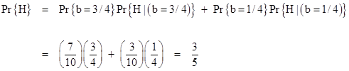
To illustrate, suppose b = 3/4 and p₀ = 7/10, which means that we initially think there's a 70% chance that the coin is biased to heads, and therefore a 30% chance that it is biased to tails. (In either case, the bias is 3:1.) Now we toss the coin, and the probability of heads on this first trial is given by

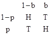
If the result of this first trial is heads, what then is our new confidence that the coin is biased to heads? The prior sample space was

If we get H on this trial we reduce the sample space to just the H portions of this table, and in that space the probability that Pr{H}=b rises to 7/8. On the other hand, if we happened to get a T on this trial, our confidence that Pr{H}=b drops to 7/16.

In general, if p is the prior probability that the coin is biased to heads, the posterior value after tossing the coin and getting heads is given by the linear fractional transformation

whereas if we get tails the posterior probability becomes

So each possible sequence of N results (such as HHTHTTHHHTH) will leave us with a certain posterior probability that can be computed by applying the two linear fractional transformations for H and T in the respective sequence. 

The likelihood of these individual strings is determined by the actual probability Pr{H}, so if Pr{H} = b the weight assigned to each string of length N containing exactly m Heads and n Tails is b^m(1–b)ⁿ whereas if Pr{H} = 1 – b the weight of such a string would be (1–b)^mbⁿ.  Therefore, the expected value (after N trials) of the probability that the coin is biased to heads depends on whether or not the coin is actually biased to heads. This stands to reason, because if our initial 'prior' is in the right direction, our posterior results won't change very much, but if our initial prior is wrong, our sequence of posterior estimates will have to migrate farther and therefore more trials will be needed to gain the same level of confidence.

Notice that the effect of m heads and n tails is the same, regardless of the order in which they occur, as can be confirmed by noting that h(t(p)) = t(h(p)) = p. In other words, the functions h(p) and t(p) are inverses of each other. Therefore, we can gather together all the C(m+n,m) strings containing exactly m heads, each of which has a weight of  either b^m (1−b)ⁿ or (1−b)^m bⁿ.

Since h(p) and t(p) are inverses of each other, the posterior probability after m heads and n tails (in any order) is the same as after m−n heads in a row. The effect of m–n consecutive Heads is given by iterating the function h(p) a total of m–n times, which has the closed form expression

This is valid regardless of whether m−n is positive, negative, or zero. Notice that if m = n the final posterior probability is simply p, meaning that if we get an equal number of heads and tails we end up with the same "belief" as at the start. Our belief varies only to the extent that m differs from n.

As noted above, there are C(m+n,m) ways of getting m heads and n tails, each with probability of either b^m(1−b)ⁿ  if  Pr{H} = b or else  bⁿ(1−b)^m  if  Pr{H} =1−b. In the first case the posterior probability after N = m+n trials is h_m−n(p₀) times C(N,m) b^m (1−b)ⁿ . Hence the discrete density function is just the binomial distribution

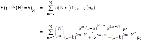
It follows that the expected value of the probability that Pr{H}=b after N trials, given that Pr{H} actually does equal b, is

On the other hand, if the probability of heads is actually 1−b, then the density function is C(N,m) (1−b)^m bⁿ, and from this we can determine the expected probability that Pr{H}=b after N trials given that Pr{H} actually does not equal b (meaning it equals 1−b). It is related to the above expression by

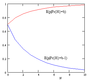
A plot of these two expectation functions for b = 3/4 and p₀ = 7/10 is shown below.

As N increases the posterior probability (of the coin being type “b”) will approach either 1 or 0 and the variance will approach 0. (The approach will be quite rapid if b is significantly different from 1/2.) The relation between these two functions can also be written in the form

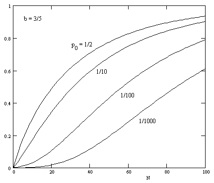
which makes it clear that the two functions are just shifted and scaled versions of a single function. Letting F(N,p₀,b) denote the left side of the above equation, it can be shown that F is unchanged if we replace p₀ with 1 – p₀ and/or if we replace b with 1 – b. A plot of this function with b = 3/5 and a range of p0 values is shown below.

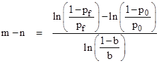
For any desired value p_f of the probability that the coin is biased to heads, we can set h_m−n(p₀) to this value and solve equation (1) for the difference m−n to give

This represented how many more heads than tails we must get to change the posterior probability (that the coin’s bias is heads) from p₀ to p_f.

Return to MathPages Main Menu