Cellular Automata

Ever since digital computers became available, people have been fascinated by the behavior of discrete fields under the action of iterative algorithms. A discrete field ϕ(j,t) consists of n ordered "locations", indexed by the integer j, at a sequence of discrete "times" t = 0, 1, 2, ...etc. Values ϕ(j,0) are assigned to each of the locations at the initial time t = 0, and the values at subsequent times are computed recursively by the n functions

for j = 0, 2,..., n−1. Thus the value at each location is a (possibly unique) function of the field values at all the locations for the preceding instant. However, in most studies the range of functions is greatly restricted so as to conform with the conventional preference for locality and homogeneity. According to the principle of locality, each F_j should be a function of just those values of ϕ(k,t) such that k is suitably "near" to j. (The measure of distance may be simply |k−j|, or it may involve a more complicated function if the locations are considered to be arranged in a multi-dimensional space.) According to the principle of homogeneity, all the F_j should be identical when expressed in terms of spatial offsets from the jth location. Homogeneity also suggests that either the locations extend infinitely in all directions, or else the dimensions are closed (e.g., cyclical), so that (in either case) there is no preferred location.

From a historical perspective it's worth noting that "cellular automata" (CA) have been in widespread use for many decades as a means of simulating complex physical phenomena. For example, to determine the potential flow field around an airfoil (such as a wing) for irrotational flow of an incompressible inviscid fluid in two dimensions, we express the Laplace equation ϕ_xx + ϕ_yy = 0 in terms of finite differences of the field values at the nodes of a uniform discrete orthogonal grid, and we find that the governing rule is simply that the value of the field at each node is the average of the values at the four neighboring locations (in the orthogonal directions). In other words, the final flow field must satisfy the relation

together with the desired boundary conditions. (A slightly generalized form of this rule may be applied if the nodes are not all equidistant.) The final flow field can be generated by assigning the desired field values at the boundary, and then iteratively computing the values at all the other nodes using the above formula until a stable condition is reached. In this way, highly complex flow fields can be generated. Likewise the solutions of many other partial differential equations (such as the Navier-Stokes equation) in one, two, or three dimensions, are routinely generated by means of suitable finite difference equations. These standard methods of numerical simulation on digital computers have been in use ever since computers became available in the 1940's, and they have been used in manual calculations for centuries. The method of finite differences makes it clear that extremely complex phenomena can be accurately simulated by the repeated application of very simple computational rules. (Incidentally, the above rule has two spatial indices, but it could be re-written with just a single index. The use of multiple indices merely simplifies the "local" references when dealing in more than one spatial dimension.)

In addition to their use for simulating partial differential equations, an arguably new aspect of simple iterative processes emerges when we examine the full range of behavior of more general iterative maps, i.e., maps that are not required to converge on any differential equation in the continuous limit. Almost everyone who has ever programmed a computer has experimented with (and been fascinated by) such algorithms, but this activity was sometimes regarded as slightly frivolous. The traditional view (at least in caricature) was that all the phenomena of nature are correctly modeled by differential equations, so the only difference equations that are relevant to the study of nature are those that correspond (in the continuous limit) to a differential equation. According to this view, all other algorithms (those that do not represent differential equations) were simply "recreational mathematics". However, there has been an increasing interest in these "frivolous" algorithms in the last few decades, leading to the idea that cellular automata may be important in their own right for the description of physical phenomena, independent of any correspondence which some of them may have with differential equations. (A similar evolution of thinking can be seen in the shift in focus from the continuous Laplace transform to the discrete "z transform" in control theory.)

Incidentally, despite the efforts of "CA" enthusiasts to free cellular automata from their role as just a means of simulating differential equations, we still find that the requirement of locality is almost invariably imposed, by making the rules strictly functions of "neighboring" cells. Locality is a fundamental and necessary characteristic of differential equations, expressing the continuity of the field, but the justification for imposing locality on abstract cellular automata is less clear. (For example, it can be shown that the wave equation can be simulated in terms of finite differences by a highly non-local algorithm.) It may be that the principle of locality has simply been carried over from the old continuous paradigm, showing how difficult it is to free ourselves from old and familiar modes of thought.

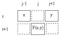
In any case, we can illustrate some of the attributes of cellular automata by considering a simple discrete field on a one-dimensional cylindrical space of n discrete locations. (The meaning of "cylindrical" is that the locations wrap around in a closed loop, so the locations j = n−1 and j = 0 are adjacent.) Applying the principles of homogeneity and locality, we focus on iterative functions ("rules") that assign a value to each location based solely on the prior values at that location and one or more neighboring location(s). (If we based the value on just the prior value at the same location, then each location would be independent of the others, and there would be no interaction.) The simplest case would be for each field value to be based on the prior values at two locations. For example, we might define each ϕ(j,t+1) as a fixed function of ϕ(j−1,t) and ϕ(j+1,t), as illustrated below.

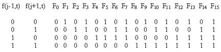
Clearly this results in two interlaced but causally disjoint networks, alternating between odd and even indices on alternate rows - a fact that will have significant implications shortly. For the time being, note that since the field has one of only two values (0 or 1), there are only four possible combinations of arguments for this function, and we can completely specify the function by assigning an output value (0 or 1) to each of these combinations. Hence there are 2⁴ = 16 distinct functions of this form, as summarized below.

Up to transposition of the two inputs and complementation of the field values, these 16 functions can be partitioned into the following seven equivalence classes:

Those functions that are symmetrical in the two arguments are the two constant functions F₀ = 0 and F₁₅ = 1 and the six familiar elementary "logic gates"

Each of the 16 functions can also be expressed algebraically. For example, F₈(x,y) = xy and F₁₄(x,y) = 1-(1-x)(1-y). The first equivalency transformation is given by transposing x and y, whereas the second is given by replacing each argument with its complement and then taking the complement.

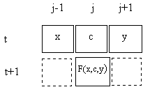
It's well known that the F₇ (NAND) gate is sufficient to synthesize all logical functions, and so too is the F₁ (NOR) gate. However, this requires the gates to be arranged and applied in suitable ways. Our simple cellular automata invokes the same rule uniformly across the entire string, and then iterates this same action on all subsequent "instants". It's easy to see that this can produce only a limited range of repetitive behaviors for any given initial string of field values. What this rule lacks is a "control code", i.e., a way of modulating the operation of the function in each instance. The simplest possible control code would be a single bit, in addition to the two "arguments" of the logic gate. Conveniently, our interlaced arrangement provides a natural place for this control code structure. For computing ϕ(j,t+1) we can use the value of ϕ(j,t) as another input, in addition to the values of ϕ(j−1,t) and ϕ(j+1,t), as shown below.

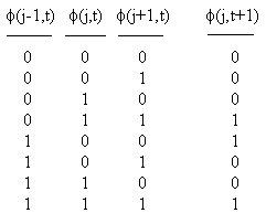
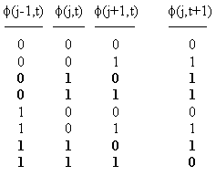
This leads us to consider a function of three field values, so the function F consists of an assignment of the value 0 or 1 to each of the eight possible sets of values in the j−1, j, and j+1 locations of the previous instant. The definition of one typical function is shown below.

The three columns on the left represent the field values at three consecutive locations at the discrete "time" t, and the right hand column gives the value assigned to of the central location at the next time, t+1. Thus there are, nominally, 256 possible rules, each corresponding to an 8-bit binary number. The particular rule above is represented by the binary number 10011000, which equals the decimal number 152, so it's convenient to refer to this as "Rule 152". If the central argument is regarded as a control code, then we see that this rule is either F₄ or F₁₀ (the 2-input functions) accordingly as the control code is 0 or 1. On the other hand, if the left hand bit is regarded as the control code, this rule is either AND or NXOR. If the right hand bit is regarded as the control code, then this rule is again F₄ or F₁₀.

Of course, if such a three-argument function is applied to each location, the "control codes" are operated upon by the results of the logical operations, and vice versa. The two originally disjoint webs (the logic gates and the control codes) now operate on an equal footing, and interact with each other, raising the prospect that a simple cellular automata of this type might actually be able to serve as a programmable computer, similar to a primitive Turing machine. For this purpose, we intuitively expect that we will need a null logic gate (for demarcation and transport) and a gate (such as a NAND gate) that is capable of synthesizing all logical functions. Arranging for the application of these two logic gates in programmed patterns, it might be possible to simulate any computable algorithm. For the "null" gate, F₁₀ is a suitable choice, because it is essentially just a pass-through gate with no logical function. (The output is simply equal to the right hand input, independent of the left hand input.) For the other logic gate, we need something like a NAND or NOR gate. Hence Rule 152 cannot perform as a general computer, because (taking the central bit as the control code) it consists of F₁₀ and F₄, and we know that the F₄ gate is not capable of synthesizing all logical functions. To construct a good candidate for a truly programmable computing function, we will combine F₁₀ with the NAND gate (F₇) and a central control code, resulting in the function shown below.

The is Rule 110, but of course we could also have used a NOR instead of the NAND, and F12 instead of F10. These alternatives (in an appropriate correspondence with the control codes) lead to Rules 124, 137, and 193. These four rules comprise an equivalence class up to reversal of the space direction and complementation of the field values (just as the NAND and NOR gates comprise an equivalence class among 2-bit functions). Judging from reviews of his recent book on the subject of cellular automata, I gather that Stephen Wolfram has made an intensive study of Rule 110, and Matthew Cook has reportedly developed a proof that this Rule can, in fact, serve as a universal computer.

In general, the 256 nominally distinct rules can be partitioned into equivalence classes, taking into account the symmetries between 0 and 1, and between the two spatial directions. Given any rule corresponding to the number N (in the range from 0 to 255), we have essentially the same rule in the opposite direction in space if we simply reverse the order of the bits representing the field values at the previous instant. The means if we apply the permutation

to the bits of N, the result will be a rule that has exactly the same effect as Rule N, but with spatial directions reversed. For example, if we apply this permutation to the bits of 152 we get 194, so the two rules corresponding to these decimal numbers are essentially equivalent. The other obvious symmetry is between the field values of 0 and 1, i.e., we can create another essentially equivalent rule by taking the complements of the prior field bits and the rule bits. Complementing the prior field bits has the same effect as applying the permutation

and then we must take the complement of each of the permuted bits of N to give an equivalent rule. Applying this transformation to 152 gives 230, whereas applying it to 194 gives 188. Consequently, the four rules 152, 194, 230, and 188 constitute an equivalence class, differing only in spatial direction and field complementation.

Of course, not all the equivalence classes contain four distinct rules, because sometimes these transformations yield the same rule as the original. The following eight rules are self-equivalent under both transformations, so they are the sole members of their respective equivalence classes:

There are also thirty-six equivalence classes containing exactly two distinct members. These are listed below. Twenty-eight are self-dual under directional reversal, whereas four (those marked with a single asterisk) are self-dual under field complementation, and four (those marked with two asterisks) are self-dual under the composition of directional reversal and field complementation.

The last set of equivalence classes are those that each contain four distinct members. The forty-four such classes are listed below.

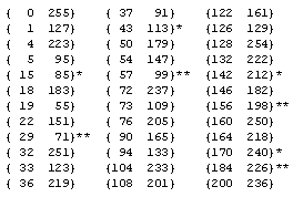
It's natural to ask which, if any, of the rules are invertible, i.e., given the field values ϕ(j,t+1) for all j, is it possible to infer the values of ϕ(j,t) from the prior instant? We find that the rules have varying degrees of invertibility. The inverted rules corresponding to each of the 256 possible rules are shown in Table 1. The only completely invertible rules are {15 85}, {51}, {170 240}, and {204}, corresponding to the "alternating" strings [00001111], [00110011], and [01010101], along with their bit reversals. In each case we find that the inverted rule is in the same equivalence class as the original, i.e., we have Inv[15] = [85], Inv[51] = [51], Inv[170] = [240], and Inv[204] = [204].

At the other extreme, there are eight equivalence classes of rules whose inverses are completely indeterminate, in the sense that no 3-bit pattern yields a unique antecedent for the central bit. Referring to these equivalence classes by their smallest member, these eight classes consist of the five quadruplets 30, 45, 60, 106, and 154, the one doublet 98, and the two singlets 105 and 150.

There are also some nearly invertible rules, i.e., those for which all but one of the 3-bit combinations yield a unique antecedent for the central bit. These consist of the two equivalence classes represented by 35 and 140. Taking Rule 35 as an example, if we have the values of ϕ(j−1,t), ϕ(j,t) and ϕ(j+1,t) we can unambiguously infer the prior value ϕ(j,t−1) for all combinations except 001. (Note that we take the least significant bit as corresponding to the highest spatial index.). This string can be preceded by either 100 or 110, which implies that ϕ(j,t−1) can be either 0 or 1. Consequently, Inv[35] is either [48] or [51]. We can actually do slightly better if we consider the next bit following 001. If the next bit is 1 (so the string is 0011), then the central antecedent bit for 001 must be 0. However, if the next bit is 0 (so the extended string is 0010), the antecedent central bit for 001 is indeterminate. Another way of expressing the degree of invertibility of the rules is shown in Table 2, which gives the possible antecedent "characters" (i.e., 3-bit strings) for each of the eight characters for a representative of each of the 88 equivalence classes.

It's also interesting to examine the distribution of k-bit strings that are produced by apply a given Rule to every possible (k+2)-bit string. With some rules, each k-bit string is yielded by exactly four (k+2)-bit strings, but with most rules there are strings that cannot possibly be produced by the application of the rule to any input string. For example, with Rule 110 we find that none of the 6-bit sub-strings 10, 18, 20, 21, and 42 can ever occur in a field to which this rule has been applied. In binary these excluded sub-strings are [001010], [010010], [010100], [010101], and [101010]. (It's interesting that the inability of Rule 110 to produce these strings does not prevent it from being a universal computing algorithm, which is by definition capable of generating any computable result. The encoding of information must be such that these strings are not needed.) In contrast, we see that for Rule 30, each of the 64 possible 6-bit substrings has the same number (four) of 8-bit predecessors.

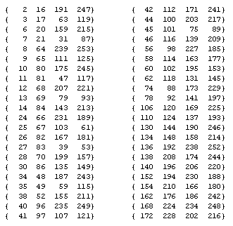
In general, let E_n(k) denote the number of excluded k-bit strings in the output of Rule n. Thus the function E_n represents a sort of "filter spectrum" for the nth rule, and it can be regarded as a measure of contraction of the rule. We find that for the 256 rules there are only 31 distinct functions E_n. Needless to say, if rules m and n are in the same equivalence class, then E_m = E_n, so there obviously could not be more than 88 distinct E functions. However, it turns out that most E functions are shared by more than one equivalence class. Table 3 shows these 31 filter spectrums, identified by representatives of the applicable equivalence classes. As can be seen in this table, the fraction of excluded strings increases with k (for most rules).

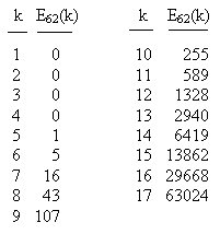
An expanded list for Rule 62 (which also applies to Rule 110), giving the number of excluded k-bit strings for k = 1 to 17, is shown below.

Notice that nearly half of all 17-bit strings are excluded. As k increases, the ratio of excluded strings to the total number of possible strings approaches 1.

In order to characterize the excluded strings for Rule 110, we can begin by examining the single 5-bit excluded string, which is 01010. Naturally this implies that no longer string produced by Rule 110 can contain this 5-bit string, so we can immediately exclude the 6-bit strings 001010, 101010, 010100, and 010101. In genenal, if the string corresponding to the k-bit binary number N is excluded, then the (k+1)-bit binary numbers N, 2N, 2N+1, and N+2^k are also excluded, simply because they contain the excluded k-bit string N. On the other hand, if a k-bit string is excluded, but it contains no excluded (k−1)-bit string, then we will call it a primitive excluded string. Obviously the 5-bit string 01010 is primitive, because there are no excluded 4-bit strings (for Rule 110). There is also a primitive 6-bit string, namely, 010010. Notice that, unlike the other four excluded 6-bit strings, this one does not contain the excluded 5-bit string. The only primitive 7-bit excluded string is 0100010, and the only primitive 8-bit excluded string is 01000010. From these cases we might be tempted to infer that there is just one primitive excluded string on each level, of the form 010...010. However, for 9-bit string there are two primitive excluded strings, the expected one, 010000010, and a new form, 010111010. Continuing to examine the primitive excluded k-bit strings for k up to 17, we find that they consist of all strings of the form

where q_j[0] signifies a string of q_j consecutive zeros. The index n signifies the number of substrings of the form [11100...], and if n = 0, there are none. The multipliers q_j are positive integers such that

Thus each primitive excluded string can be expressed by the values of q_j. For example, the primitive excluded string 0100001110111000111010 (which has k = 22 and n = 3) corresponds to the q_j values {q₀,q₁,q₂,q₃} = {4,1,3,1}. The number of primitive excluded k-bit strings for Rule 110 with k = 1, 2,...etc. are 0, 0, 0, 0, 1, 1, 1, 1, 2, 3, 4, 5, 7, 10, 14, 19, 26, ... and so on. These numbers form a linear recurring sequence, satisfying the forth-order recurrence s_n = s_n−1 + s_n−4.

We can also examine the primitive excluded strings for each of the other rules. Naturally they fall into just 31 distinct classes, corresponding to the sets of rules that share a common E function. Table 4 lists the numbers of primitive excluded strings for each of the 31 distinct E functions. We note that rule classes 37 and 62 are the only ones with a monotonically increasing number of primitive excluded strings. Also, rule classes 0, 4, 7, 19, 29, and 50 each have only one primitive excluded string. Thirteen other rule classes have only a finite number of primitive excluded strings. Rule classes 27 and 58 are unique in each having a constant number of primitive excluded k-bit strings for each sufficiently large k. On the other hand, rule class 46 has precisely one primitive excluded k-bit string for every odd k (greater than 1) and none for any even k. For the remaining nine rule classes the number of primitive excluded strings of length k evidently increases without bound as k increases, eventually roughly doubling on each step.  For a more detailed discussion of the number of excluded strings (primitive and total) for each of the rule classes, including recurrence relations and closed form expressions for these numbers, see the note on Impossible Strings for Cellular Automata.

We can also examine the k-bit strings that are nearly excluded, i.e., that are produced by the application of the given rule to just one specific (k+2)-bit string. More generally, we can determine how many (k+2)-bit strings are the predecessor of each k-bit string. We find that many rules which share the same E function also share the same distribution of predecessors, but this is not always the case. In other words, some rules that share the same E function nevertheless have a different distribution of predecessors. There are 51 distinct predecessor valence distributions for 6-bit strings, as shown in Table 5.

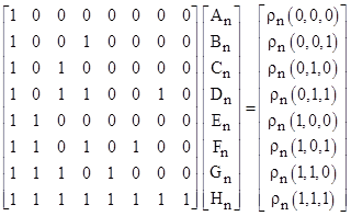
We previously described how a particular rule can be specified by means of a table, which assigns to each 3-bit string either a 0 or 1 as the output, i.e., the central bit at the subsequent instant. It's also possible to express rules algebraically, and this form of expression not only clarifies the equivalence transformations, it immediately generalizes the functions to arbitrary arguments and outputs (not restricted to the set 0,1). In general we can express a rule by an equation of the form

for constants A,B,...,H. In this equation we have let ϕ₁, ϕ₂, and ϕ₃ denote the three field values at the current instant, and ϕ₂⁺ denotes the central field value at the next instant. This is the most general algebraic function that is linear in each of the three arguments. For the nth rule we will denote the right hand side of the above equation by ρ_n(ϕ₁,ϕ₂,ϕ₃). To find the coefficients of ρ_n for any given n we simply need to solve the matrix equation

The determinant of the square matrix is −1, so we can simply invert this matrix and multiply through to give the coefficients for the algebraic form of any rule. Following are the algebraic expressions for a few particular rules:

If we let α(n) denote the rule equivalent to n transformed by reversing the spatial directions, and if we let β(n) denote the rule equivalent to n transformed by reversing the field values 0 and 1, then the transformations can be expressed in terms of the respective polynomials as

Clearly each of these transformations has period 2. These transformations and their compositions induce the 88 equivalence classes described previously. In other words, applying either of these transformations to a rule produces another rule in the same equivalence class. The polynomials for representative rules of several equivalence classes of particular interest are shown below.

Although these polynomials were derived based on the assumption that the field can take on only the values 0 or 1, they can be applied to more general sets of numbers. Of course, we require closure of the set under these operations. Some of the rules induce non-trivial sets of field values. For example, if we begin by allowing the field to take on any of the values −1, 0, or +1, then closure under ρ₉₀ implies the minimal set of field values ..., −1093, −344, −121, −40, −13, −4, −1, 0, 1, 2, 5, 14, 41, 122, 365, 1094, ... However, most of the non-trivial rules induce the complete set of integers beginning from the initial set {−1, 0, +1}.

A more natural extension of the field values is to allow them to take on any real value on the interval from 0 to 1. On this basis they can be regarded as probabilities (or as projection parameters). We're assured that each rule maps from this range to itself, because each rule is linear in each of the arguments, and the output ranges between 0 and 1 as each argument is individually varied from 0 to 1 (or else the function is independent of the argument). However, the sum total of the field values is, in general, not conserved under the action of a rule, so in order to interpret the field values as probabilities we would need to re-normalize the values on each iteration, so that they always sum to 1. Beginning with a string containing just a single 1, the result is a diffusing distribution, which may either be either stationary or moving, depending on which rule is applied. This diffusion makes it intuitively clear that most rules could not be invertible, because if they were, it would be possible to reverse the diffusion of a wave and reconstruct the original spike.

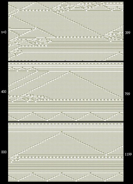
It's customary to apply just a single rule, but since the rules fall into natural equivalence classes, we can also consider algorithms that apply all the elements of a single class. This is consistent with the idea of having no preferred direction or field value. For example, consider the equivalence class consisting of the rules 110, 124, 137, and 193. (We focus on this particular equivalence class because, when viewed as an elementary 2-input logic gate with a central control code, rule 110 functions as either a NAND gate or as F₁₀, which is precisely the pair of logic gates which enables us to synthesize the most general functionality.) If we apply these cyclically in the order 110, 137, 193, 124, 110, ... etc., we find some fascinating results. Beginning with an initial string (loop) consisting of repetitions of {0011}, the application of the 110.137.193.124 rule yields a uniform "background" with the small-scale periodic pattern {0011}, {1011}, {1001}, {0001}, {0011}, and so on. Now, in the initial string we can place various kinds of anomalies, which may be stationary "barriers" or propagating "objects", and we find that these objects interact with each other and with the barriers in an amazing variety of ways. The image below is just one sample of the kinds of behavior that arises in just a 206-bit circular string under the action of the 110.137.193.124 rule.

Notice in particular the detailed activity near the upper edge of the strip at about t = 400 to 500, including the small-scale zig-zag pattern on the blank background that is intercepted and annihilated by the object coming in from below. The initial (t = 0) string of 206 bits for this case in hexadecimal characters and 2 binary bits was

33633 33337 33B73 33333 32C64 66666 66676 656E6 66676 6666E 6 [01]

It's quite easy with this algorithm to "program" barriers and bouncing balls, and the frequency and phase of each such "channel" is established by the distance between the barriers and the initial position of the contained object. In addition, channels can interact with each other at the boundaries when the objects strike their respective sides of the boundaries simultaneously (as illustrated in the example above). Based on these capabilities alone, it's clear that this algorithm can mimic a universal Turing machine, but there are actually many more kinds of interactions that could be exploited for theoretical computational purposes. The algorithm seems to possess an almost inexhaustible versatility.

For more on cellular automata, see the articles

Impossible Strings for Cellular Automata

Function 34776

Global Reversibility of Cellular Automata

Return to MathPages Main Menu