Schwarzschild Coordinate Time

The essentially unique spherically symmetrical solution of Einstein’s field equations can be expressed in explicitly stationary form, i.e., such that the metric coefficients are independent of the time coordinate. This gives the Schwarzschild metric, which, for purely radial paths, is simply

This line element implies a genuine singularity in the manifold at r = 0 (where the curvature goes to infinity), and hence there is a fixed point of reference for the labeling of the radial coordinate. However, the Schwarzschild time coordinate t appears only as the squared differential, so there is no fixed point of reference to establish the absolute value (nor even the sign) of t at any event. Thus, given any labeling of events (t, r) that satisfies the above metric, the alternative labeling (±t + k, r) for any constant k also satisfies the metric.

Of course, the coefficients of the metric (1) are also singular at r = 2m, but the manifold itself is not singular at that location, as shown by the fact that all the components of the curvature tensor remain finite and continuous there. Hence geodesic paths can be continued smoothly and unambiguously across that boundary. Indeed, over a sufficiently small region around r = 2m the spacetime manifold is (locally) indistinguishable from flat spacetime, and the line element is approximately given by the Minkowski metric in terms of suitable coordinates. (This is implied by the equivalence principle.) The singularity of the Schwarzschild metric coefficients at r = 2m signifies that the Schwarzschild coordinates (t,r) are not suitable at that location, just as the singularity in the longitude and latitude coordinates at the North Pole signifies that those are not suitable (useful) coordinates at that location.

Nevertheless, the Schwarzschild time coordinate t has absolute physical significance in the sense that it is the essentially unique time coordinate in terms of which the metric coefficients (for a spherically symmetrical field) are stationary. For this reason, it’s interesting to examine the expressions for continuous geodesic paths in terms of the Schwarzschild coordinates, on both sides of the coordinate singularity at r = 2m. Not surprisingly, there is an ambiguity in the Schwarzschild time coordinate as we pass from outside to inside this boundary. This was to be expected, because t appears in the line element only as a squared differential, and it is singular at this boundary.

As discussed in the note on radial paths in a spherically symmetrical field produced by a body of mass m, the geodesic equations in Schwarzschild geometry imply that the coordinate time t is related to the proper time τ along the path of a particle falling freely (and radially) from rest at the location r = R by

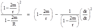
Dividing through the line element (1) by (dt)² and substituting the above expression for dt/dτ, we get

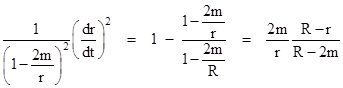
Re-arranging terms and simplifying, this leads to

With a bit more re-arrangement we arrive at

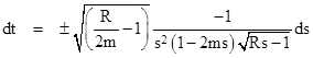
We can simplify the integration by making the change of variables s = 1/r, in terms of which the above relation can be written as

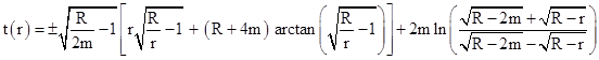
To assign a value of t to each value of r for the free-fall path from r = R (where we arbitrarily define t = 0) down to r = 0 we must integrate this equation over that range, but a complication arises due to the fact that the integrand on the right side is infinite at r = 2m (which is to say, at s = (2m)^–1). Of course, this doesn’t prevent us from evaluating the difference in the anti-derivative at s = 1/R and s = 1/r for any desired value of r. Carrying this out, replacing s with 1/r, and simplifying, we get

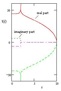
However, due to the singularity of the integrand at r = 2m, the argument of the logarithm is negative for r less than 2m. As a consequence, the value of t(r) given by this formula for r less than 2m is complex, because the logarithm of a negative number (by analytic continuation) is augmented by πi plus any integer multiple of 2πi. The figure below shows the real and imaginary parts of t(r) for this free-fall trajectory for r = R down to r = 0, with the values R = 10 and m = 1.

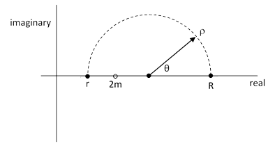
One way of arriving at this result is by complex integration. We need to integrate equation (2) along the radial axis from the apogee at R to the variable r, but in order to avoid passing through the singularity at r = 2m we must integrate along a path in the plane of complex values of r. We know from the theory of complex integration that the integral along any two paths between two given points is the same, provided the paths do not enclose any singularities. Hence every path that passes above the singularity (and not below) will give the same result. The figure below shows one convenient path along which we can integrate from R to any lesser radial location without passing through the singularity.

The semi-circular path from R to r is given by

as θ ranges from 0 to π. Making this change of variables in equation (2) and integrating over θ, we get the same expression for t(r) as given above. Of course, if we chose a path of integration in the lower half plane, the resulting imaginary part would be -2m(πi) instead of +2m(πi). If we chose a path that circled completely around the singularity k times in the counter-clockwise direction, we would get an additional 2m(2kπi) contribution to the imaginary part of t(r). In this sense, t(r) is a multi-valued function. Strictly speaking, this is true even for values of r greater than 2m, but in that case the imaginary part is an even integer multiple of 2m(πi), which we can take to be zero, whereas when r is less than 2m the imaginary part of t(r) is an odd integer multiple of 2m(πi).

Is there any physical significance to the imaginary offset of t(r) in the region r < 2m? Recall from the previous discussion that, since the t coordinate does not appear in the metric coefficients, the absolute value of t has no significance. We can add an arbitrary offset to all the t labels, and they will still satisfy all the requirements of the metric. Of course, this offset must be constant in order to maintain continuity of the t coordinate and avoid upsetting the metric, in which the total differential dt appears. However, the t coordinate is unavoidably discontinuous at r = 2m, even under analytic continuation, because the imaginary part changes abruptly for real values of r on opposite sides of that point, as shown in the figure above. Furthermore, depending on how many times the path of integration loops around the singularity, the step change in the imaginary part of t(r) can be arbitrarily large, and either positive or negative. Likewise the value of t(r) in the outer region r > 2m can be offset by even integer multiples of 2m(πi), so its imaginary part can be arbitrarily large, and either positive or negative.

The usual conclusion is that the arbitrary constant offsets for the regions r > 2m and r < 2m are independent, and so we are free to subtract an odd multiple of 2m(πi) from the interior values of t(r), and thereby take t(r) to be real-valued for all r. Recalling that the logarithm of an arbitrary complex number z = re^iθ is

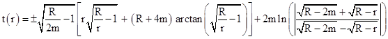
where k is an arbitrary integer, and that the principle branch is with k = 0, we can accomplish the offset of the interior value of t(r) simply by taking the absolute value of the argument of the logarithm, leading to the textbook result

This certainly gives a valid and convenient labeling of the t coordinates, but it may be worth noting that it is not unique. We can obviously add an arbitrary constant to this expression without affecting its validity. This just amounts to choosing a zero point for the time coordinate, which, as discussed previously, is arbitrary. As written, the equation gives t(R) = 0, so it assigns the value t = 0 to the apogee of the radial trajectory, but we could just as well define t = 0 at any other point. Moreover, we’ve seen that this free offset is independent for the values of t(r) in the ranges r < 2m and r > 2m. Therefore, in terms of the parameters

the most general expression for t(r) consists of two parts which can be written as

where C₁ and C₂ are arbitrary complex constants, defining the coordinate offsets for the ranges inside and outside the point r = 2m respectively.

The freedom to independently choose constant offsets (and the signs of Q) for the t coordinates inside and outside the radius r = 2m is entirely consistent, both with the continuous geodesics passing through that radius (as we’ve shown above) and with the Kruskal coordinates. The relation between the Schwarzschild (t,r) and Kruskal (u,v) coordinates (for the fully extended Schwarzschild spacetime) is usually given for the four regions as shown below.

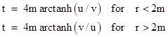
On this basis, noting that r > 2m for regions I and III, and r < 2m for regions II and IV, the inverse transformations are

and

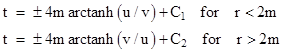
However, this isn’t fully general, because we know the t coordinate values can all be offset by any constant, and their signs can be reversed, without having any effect. Thus we could certainly add a constant C to each of the above expressions for t, as well as to reverse any of the signs of t. Furthermore, noting that the t labels are discontinuous at r = 2m (where v/u = ±1), we are free to add different constants, C₁ and C₂, to the above expressions for t for the ranges r < 2m and r > 2m respectively. Hence the more general relation between the Schwarzschild time coordinate t and the Kruskal coordinates u and v is

for arbitrary (finite) complex constants C₁ and C₂. This clearly has no effect on the form of the metric for the u,v coordinates, because that metric is derived from the above expressions by first taking the total differentials to give dr and dt as functions of du and dv. When we take the differentials of the expressions for t, any constants drop out. Thus, regardless of the values of C₁ and C₂, we get the relations

Substituting these differentials into the Schwarzschild metric (1) and simplifying, we arrive at the metric in terms of Kruskal coordinates

which is non-singular for all radial locations except r = 0. Thus the inclusion of the constant offsets C₁ and C₂ (and the alternate signs) has no effect on the form of the Kruskal extension. This simply confirms the fact that we can shift and/or negate the t labels inside and outside the radius r = 2m independently. The usual assumptions are merely the most convenient conventions, giving the simplest expressions.

Return to MathPages Main Menu