Open-Loop and Closed-Loop Markov Models

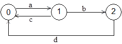
The essential differences between open-loop and closed-loop Markov modeling methods can be illustrated by a simple 3-state model {S₀, S₁, S₂} where S₀ is the full-up condition, S₁ is the partially failed condition, and S₂ is a complete failure (a "shutdown"). Failure transitions S₀→S₁ and S₁→S₂ are exponentially distributed with rates "a" and "b" respectively. Periodically (every T hours) all partially failed systems are repaired. If a system experiences a shutdown it is repaired immediately and returned to service. Our objective is to determine the mean time between shutdowns as a function of the inspection/repair interval T.

A closed-loop Markov model for this system is shown below.

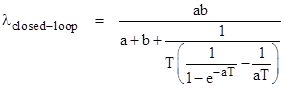
The repair transition S₁→S₀ is treated as exponential with rate c = 1/MTTR, where MTTR is the mean time to repair of partial faults. If T is sufficiently small the value of MTTR is approximately T/2, but to cover the whole range of possible T values we need to use

Strictly speaking the transition S₂→S₀ is also treated as exponential (with rate "d"), but since the rate of entering S₂ is independent of the rate of leaving S₂, this rate always drops out of the final result.

The steady-state solution of the closed-loop model is found by solving the equilibrium equations

which give

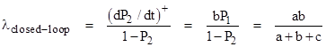
From this we can compute the rate of entry into S₂ as follows

(The symbol (dP₂/dt)⁺ signifies the positive component of dP₂/dt, because we want the rate of entry into S₂.) Setting c = 1/MTTR we have the result

Notice that as T increases to infinity the rate approaches ab/(a+b), which we recognize as the correct rate assuming partial failures are never repaired.

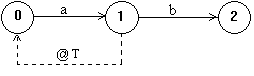
The open-loop model for this system is shown below.

The idea of this approach is to simulate the actual periodic repair process (rather than treating the transition S₁→S₀ as exponential) by running the model without repairs for an interval of length T, and then inferring the effective shutdown rate from the probability of the shutdown state at time T.

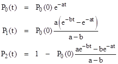
Assuming P₂(0) = 0 (i.e., the partial failure state is empty at t = 0) the dynamic solution of the open-loop model (with d = 0) is

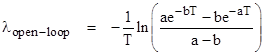
A simple method of approximating the MTBF of this system would be to set P₀(0) = 1 and compute the value of P₂(T). Then if we assumed this probability accumulated in S₂ at a constant rate λ, we could solve the equation P₂(T) = 1 – e^–λT for λ, which gives

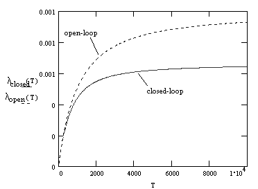
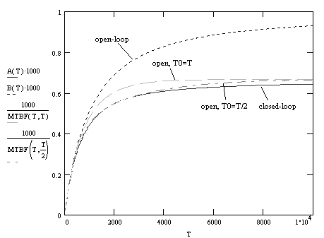
This value of λ_open-loop is plotted along with λ_closed-loop in the figure below. (For illustration purposes we have taken a = 0.002 and b = 0.001)

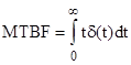
As can be seen, the two values agree for small T, but they differ as T increases. We know the closed-loop model gives the correct asymptotic rate as T increases (which can be verified using numerical simulation), so there is evidently something wrong with the simple open-loop approach just described. The main problem is the assumption that the probability accumulates in S₂ at a constant rate, which is not generally the case. The initial shutdown rate is quite low (because S₁ starts out empty) and then increases. In general, two different probability density functions that give equal values of P₂(T) can have different MTBFs, because of how the failures are distributed during the interval T. This means we cannot actually infer the true MTBF from the open-loop value of P₂(T) alone. For non-constant failure rates the only way to determine the actual mean time for a system to fail is by integrating t times the failure density function δ(t) using the formula

Then the "effective failure rate" can be defined as 1/MTBF. Unfortunately the density function for a system with periodic repairs is somewhat complicated. The probability of State 2 as a function of time during a single inspection interval is

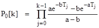
where t = 0 at the start of this interval. Letting P_j[k] denote the value of P_j(0) at the start of the kth period, we have P₂[k] = 1 – P₀[k] (because the partial failure state is empty at the start of each interval). Also, we have P₀[0] = 1, and the above equation implies that

for all k > 0, where Tj is the duration of the jth period. Fortunately, all the T_j except possibly T₀ are of equal duration, which we will call simply T. Therefore, if we define

we have

for all k>0. For convenience let q₀ denote q(T₀) and q denote q(T). Then the probability density function for the initial period T₀ is

and for all subsequent periods the density function is

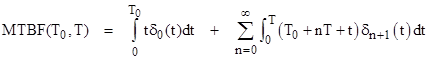
The MTBF of the system is then given by

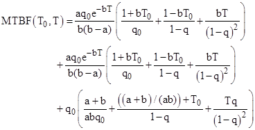
Evaluating the integrals and summing the resulting geometric series we finally arrive at the result

Taking a strict open-loop approach (neglecting the repair transition shown as a dotted line in the open-loop schematic), the system always starts at t = 0 at the beginning of the initial inspection/repair interval, and so we have T₀ = T. The resulting effective shutdown rate is shown in the figure below along with the closed-loop rate.

The match is a little better than the previous open-loop method - at least now they both have the correct asymptotic rate as T goes to infinity. However, the open-loop method approaches the asymptote much more quickly than the closed-loop method. Which method is correct?

The answer is that both methods are correct, but they represent different things. The open-loop method (without the dotted repair transition) always begins the first inspection/repair interval at t = 0. The MTBF of the system in those circumstances is as given by the open-loop model with T₀ = T. However, in practice we don't re-synchronize our inspection/repair cycle each time we have a shutdown. For example, if a system fails half-way through our inspection interval we fix it and return it to service, so it's initial inspection interval (on the way to it's next failure) is only half of the normal interval. Since a shutdown can occur anywhere during the interval, the actual value of T₀ can be anything from 0 to T, with a mean value of T/2.

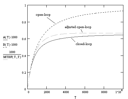
The figure below shows the open-loop rate, taking T₀ = T/2, along with the closed loop rate. As can be seen, the results of the open-loop method with T₀ = T/2 are almost identical to the closed-loop prediction. This result is confirmed by numerical simulation of the system with periodic inspections every T hours, assuming the inspection cycle is not re-synchronized with each shutdown.

Thus we can achieve fairly consistent results using the open-loop with strictly periodic (as opposed to exponential) repairs. This shows that there is not much difference between periodic and exponential repair transitions. Of course, if we're willing to represent the repair transition from S₁ to S₀ as exponential with constant rate c = 1/MTTR, as we did with the closed-loop model, then we can get exactly the same answer as we got using the closed-loop model. On this basis the open-loop model is as shown below.

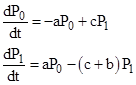
Since P₂(t) = 1 – P₀(t) – P₁(t) the two governing equations are simply

The characteristic roots of this system are

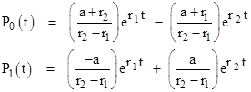
 With the initial condition P₀(0) = 1 the solution is

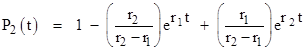
Consequently the cumulative probability function for state 2 is

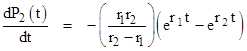
and the probability density function for entering state 2 is the derivative of this, i.e.,

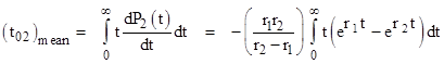
The mean time to reach state 2 from state 0 is given by the integral

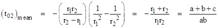
Evaluating the integral give

which is exactly equal to the reciprocal of the closed-loop failure rate.

In summary, the it is usually possible to represent periodic repairs as exponential transitions, and it is possible to achieve consistent results using either the closed-loop or the open-loop approach. However, the open-loop approach generally requires much more effort, and for complicated systems it quickly becomes impractical.

Return to MathPages Main Menu