Iterative Isoscelizing

In the xy plane consider a triangle whose base coincides with the segment (0,0) to (2,0) of the x axis, and whose height is h. The area of the triangle is A = h. Without changing the area, we can place the upper vertex at (1,h), resulting in an isosceles triangle with area A. Now, proceeding clockwise around the perimeter, we can hold the next edge fixed as the base, and re-position the opposite vertex to give an isosceles triangle of the same area. We can continue in this way, iteratively "isoscelizing" the triangle, taking consecutive edges clockwise around the perimeter as the bases. (Steve Gray asked if anything was known about this iteration.)

It's easy to see that this process converges on a fixed equilateral triangle. If the edge lengths of the original triangle are a,b,c, then by Heron's formula the squared area of the triangle is

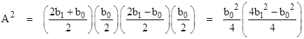
Holding the area constant and taking edge b as the fixed base with length b = b₀, we isoscelize the triangle by setting a = c = b₁, where b₁ will be the fixed base length on the next iteration. Making these substitutions, we have

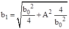
Solving this for b₁ gives

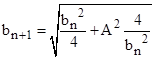
The same formula applies recursively, so in general the sequence of base lengths satisfies the recurrence

The sequence converges on the stationary condition b_n+1 = b_n, which gives the asymptotic relation

which represents the final equilateral triangle.

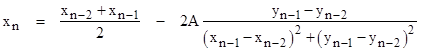
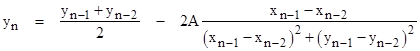
The above analysis shows only the behavior of the successive edge lengths, but we can also consider the absolute position and orientation of the final (asymptotic) equilateral triangle. Given the coordinates (x_n,y_n) and (x_n+1,y_n+1) of the two vertices on the base of a triangle of area A, the coordinates of the remaining vertex of the isosceles triangle on that base are given by

Taking the initial vertices (0,2) and (0,0), and an arbitrary (non-negative) area A, these equations can be used to perform iterative "isoscelization" until arriving at a fixed equilateral triangle. The coordinates of the centroid at any given stage are

Let X(A) and Y(A) denote the coordinates of the centroid of the asymptotic triangle given by the recurrence for any given area A. Clearly with A = 0 we have all three vertices on the y axis, and the first isoscelized vertex on the base (0,2) to (0,0) is just the midpoint (0,1). We then hold the vertices (0,0) and (0,1) fixed and place the next vertex at the midpoint (0,1/2). The next point is (0,3/4), then (0,5/8), and so on. This recurrence converges on the point (0,2/3), so we have X(0) = 0 and Y(0) = 2/3.

Another simple case is with the area A = √3, which corresponds to an initial isosceles triangle on the base from (0,2) to (0,0) that is already equilateral. Consequently it is a fixed point of the iteration, and the asymptotic centroid is simply given by X(√3) = 1/√3 and Y(√3) = 1.

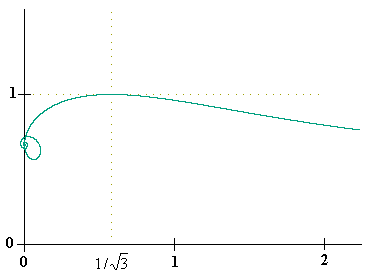
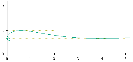
Numerically we can apply the basic coordinate recurrence and plot the locus of asymptotic centroid positions as a function of A. The figure below show such a plot for A ranging from 0 to 4.

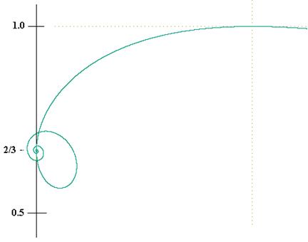
This confirms that the asymptotic centroid begins at (0, 2/3) for A = 0, and passes through the point (1/√3, 1) , which corresponds to the area A = √3. It also shows that for small values of A the locus loops around the point (0,2/3). It's interesting to focus in on this region, as shown in the figure below.

Expanding the view still more, we have the plot shown below.

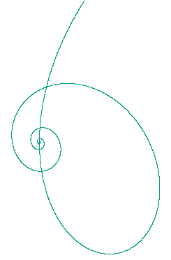
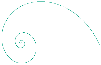
Zooming in still further, we find that the locus of centroids becomes an apparently logarithmic spiral, as shown below.

Incidentally, the locus curves around and passes precisely through the "origin" point (0,2/3) for an area of 1/√3 (as seen in the previous views).

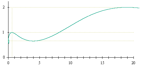
Going in the other direction, we can step back and take a larger view of the original plot, as shown below.

Zooming back another level gives the view

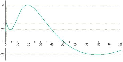
and zooming back still one more level gives the view

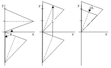
It's apparent from these views that the locus has self-similar and logarithmic qualities. For example, in the spiral region, for each rotation of π radians about the "center", the area A increases by about a factor of 4, and the radius increases by about a factor of 2. Similarly in the region of large A, the X coordinate of the maxima and minima increases roughly as (4/3)A, whereas the Y coordinates are asymptotically related to A by Y² = A/36. As a result, the envelope of this locus approaches a sideways parabola of the form X = 48Y². To understand this self-similar behavior, notice that for any given value of the area A, our initial triangle (prior to applying the isoscelizing iteration) has the three vertices (0,2), (0,0), and (A,1), and the length L of the two equal sides satisfies the relation L² = A² + 1. Suppose we rotate the triangle in the plane clockwise about the origin through the angle q that aligns the lower side of the triangle with the y axis, as indicated in the left-hand figure below.

Once the triangle has been rotated, we can raise it by an amount L in the y direction, so that the lower vertex is at the origin, as shown in the middle figure above. Then we need only re-scale the triangle by a factor of 2/L, as shown in the right-hand figure, to make the "base" along the y axis map to the segment (0,2) to (0,0). Of course, this re-scaling causes the area of the triangle to be reduced by a factor of 4/L², so the area of this transformed triangle is

If we happen to the asymptotic centroid position coordinates X(A') and Y(A') for this transformed area, we can then apply the reverse transformation, re-scaling by a factor of L/2, shifting down by L, and rotating in the counter-clockwise direction through the angle θ, to give the centroid position coordinates X(A) and Y(A) of the original area. Thus we have

Using the identities

as well as the expression for A' in terms of A, we have the following functional equations for X(A) and Y(A):

To demonstrate, we can consider the three areas for which the centroid position is already known. First, with A = 0 we have A' = 0, and we already know that X(0) = 0 and Y(0) = 2/3, so we can confirm the consistency of these equation as follows

For a second example, consider the case A = √3, for which we have A' = √3. The asymptotic centroid coordinates are X(√3) = 1/√3 and Y(√3) = 1, and the consistency of the functional equations is demonstrated as follows

For a slightly less trivial case, we can consider A = 1/√3, for which we have A' = √3. Using the known values of X(√3) and Y(√3), the functional equations give

This confirms our earlier assertion that the locus of centroids passes through this "origin" point for A = 1/√3 as well as for A = 0.

The functional equations also explain our earlier observations about how, for very small values of A, where the centroid locus is essentially just a logarithmic spiral, each rotation of the locus through an angle of p doubles the radius and corresponds to a quadrupling of the area. Notice that, for extremely small values of A, the functional equations can be approximated by the simplified form

Looking at the X equation, we see that a point on a right-most extremum of the spiral is sent to a left-most extremum at twice the radius when A is increased by a factor of 4.

At the other extreme, with very large values of A, the functional equations approach the simplified form

As A increases, the values of X(4/A) and Y(4/A) become small, although they are multiplied by A/2 in these expressions, yielding a net increase. However, the dominant term is given by the A component of X(A), which explains why we found numerically that X(A) is on the order of A for large A. (Specifically, X(A) approaches (4/3)A.)

We can also examine other interesting aspects of this process, such as the angular orientation of the asymptotic equilateral triangle as a function of A, and we can map the loci of the three vertices of the asymptotic triangles as functions of A. We can also consider, formally, the results of extending this process to negative values of the area.

Return to MathPages Main Menu