|
Old Notes on Curvature |
|
|
|
The extrinsic curvature of a surface embedded in a higher dimensional space can be defined as a measure of the rate of deviation between that surface and some tangent reference surface at a given point. It's worthwhile to start with a 1-dimensional example. At any point on a 1-dimensional surface (a curve) we can set up an "xy" orthogonal coordinate system in the plane of the curve at that point such that the x axis is tangent (and the y axis is perpendicular) to the curve. If we express the curve in the neighborhood of that point by a function y = f(x) then our point is at the origin (0,0) of these coordinates, and the curvature at this point is simply the second derivative of f(x) evaluated at x = 0. |
|
|
|
The general power series expansion of a function is |
|
|
|
|
|
|
|
but since we explicitly set up our coordinates so that the curve passes through the origin, and is tangent to the x axis at this point, we know that c0 = c1 = 0, so the expansion of our curve about this point will be of the form |
|
|
|
|
|
|
|
Furthermore, the 2nd derivative is |
|
|
|
|
|
|
|
and evaluating this at x = 0 gives simply f ″(0) = 2c2. This shows that only the 2nd-order term is significant in determining curvature, so we can just represent our curve in the parabolic form f(x) = ax2 with curvature 2a. |
|
|
|
Now suppose we are given a function f(x) representing a plane curve in terms of some arbitrary xy coordinate system on the plane, and we want to determine the curvature at particular point P on this curve. We can do this by expressing the function in terms of a rotated set of coordinates tangent to the function at P, and then evaluating the 2nd derivative at that point. It's not hard to show that the result can be expressed in terms of the original (arbitrary) coordinates as |
|
|
|
|
|
|
|
This really just amounts to correcting the 2nd derivative when it's evaluated in a coordinate system whose x axis is not tangent to the function at the point in question. Note that if the x axis is tangent to the function at x, then fʹ(x) = 0 and the formula reduces to simply C(x) = f ″(x). |
|
|
|
The curvatures of a few common functions are listed below: |
|
|
|
Curve f(x) curvature |
|
___________ ____________ ___________________ |
|
|
|
parabola x2
|
|
|
|
circle |
|
|
|
logarithm ln(x)
|
|
|
|
hyperbola 1/x
|
|
|
|
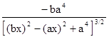
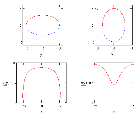
ellipse |
|
|
|
It's interesting that the equation for the curvature of an ellipse as a function of axial position actually extends beyond the ellipse itself, as shown for the two principal axes in the figures below |
|
|
|
|
|
|
|
Now let's consider the extrinsic curvature of a two-dimensional surface in space. At any given point on the surface we can construct an orthogonal "xyz" coordinate system such that the xy plane is tangent to the surface and the z axis is perpendicular to the surface at that point. In general the equation of our surface can be expanded about this point into a polynomial giving the "height" z as a function of x and y. As in the 1-dimensional case, the constant and 1st-order terms of this polynomial will be zero (because we defined our coordinates tangent to the surface with the origin at the point in question), and the 3rd and higher order terms won't affect the second derivative at the origin, so we can represent our surface by just the 2nd-order terms of the expansion, i.e., |
|
|
|
|
|
|
|
The second (partial) derivatives of this function with respect to x and y are 2a and 2c respectively, so these numbers give us some information about the curvature of the surface. However, we'd really like to know the curvature of the surface evaluated in any direction, not just in the x and y directions. (Note that the tangency condition uniquely determines the direction of the z axis, but the x and y axes can be rotated anywhere in the tangent plane.) |
|
|
|
In general we can evaluate the curvature of the surface in the direction of the line y = kx for any constant k. The equation of the surface in this direction is simply |
|
|
|
|
|
|
|
but of course we want to evaluate the derivatives with respect to changes along this direction, rather than changes in the pure x direction. Parametrically the distance along the tangent plane in the y = kx direction is s2 = x2 + y2 = (1 + k2) x2, so we can substitute for x2 in the preceding equation to give the value of f as a function of the distance s |
|
|
|
|
|
|
|
The second derivative of this function gives the curvature of the surface in the "k" direction: |
|
|
|
|
|
|
|
The directions of extreme (min and max) curvature are found by setting the derivative of C(k) to zero, which gives |
|
|
|
|
|
|
|
where q = (c – a)/b. The two roots are k1 = q + (1+q2)1/2 and k2 = q – (1+q2)1/2. Since the product of the two roots is –1, they are the negative reciprocal of the other, so the lines of min and max curvature are of the form y = (k1)x and y = (–1/k1)x, which shows that the two directions are perpendicular. Substituting the two "extreme" values of k into the equation for C(k) gives (Note 1) the two "principal curvatures" of the surface |
|
|
|
|
|
|
|
The product of these two is called the "Gaussian curvature" of the surface at that point, and is given by |
|
|
|
|
|
|
|
which of course is just the (negative) discriminant of the quadratic form ax2 + bxy + cy2. For the surface of a sphere of radius R this quantity equals 1/R2. (Note 2) |
|
|
|
Another measure of the curvature of a surface is called the "mean curvature", which, as the name suggests, is the mean value of the curvature over all possible directions. Since we want to give all the directions equal weight, we insert tan(θ) for k in the equation for C(k) and then integrate over θ, giving the mean curvature |
|
|
|
|
|
|
|
Of course, we could also infer this mean value directly as the average of C1 and C2 since C is symmetrically distributed. |
|
|
|
Notice that the mean curvature occurs along two perpendicular directions, and these are oriented at 45 degrees relative to the "principal" directions. This can be verified by setting the derivative of the product C(k) C(–1/k) to zero and noting that the resulting quartic in k factors into two quadratics, one giving the two principal directions, and the other giving the directions of the mean curvature. (The product C(k) C(–1/k) is obviously a maximum when both terms have the mean value, and a minimum when |
|
the terms have their extreme values.) |
|
|
|
Examples of surfaces with constant Gaussian curvature are the sphere, the plane, and the pseudo-sphere, which have positive, zero, and negative curvature respectively. (Negative Gaussian curvature signifies that the two principal curvatures have opposite signs, meaning the surface has a "saddle" shape.) |
|
|
|
Surfaces with vanishing mean curvature are called "minimal surfaces", and represent the kinds of surfaces that are formed by a "soap films". Until recently the only complete and non-self-intersecting minimal surfaces known were the plane, the catenoid, and the helicoid, but a few years ago Celso Costa, David Hoffman and Bill Meeks discovered an infinite family of such minimal surfaces. |
|
|
|
The above discussion was based on extrinsic properties of surfaces, i.e., measuring the rate of deviation between one surface and another. However, we can also look at curvature from an intrinsic standpoint, in terms of the relations between points within the surface itself. For example, if we were confined the surface of a sphere of radius R, we would find that the ratio Q of the circumference to the "radius" of a circle as measured on the surface of the sphere would not be constant but would depend on the circle's radius r according to the relation Q = π (R/r) sin(r/R). Evaluating the second derivative of Q with respect to r in the limit as r goes to zero we have |
|
|
|
|
|
|
|
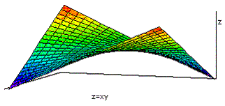
Thus we can infer the radius of our sphere entirely from local measurements over a small region of the surface. The results of such local measurements of intrinsic distances on a surface can be encapsulated in the form of a "metric tensor" relative to any chosen system of coordinates on the surface. To illustrate this concept, consider the simple surface given by the equation z = xy/R where R is a constant. A plot of this surface is shown below: |
|
|
|
|
|
|
|
This function is single-valued over the entire xy plane, so it's convenient to simply project the xy grid onto the surface and use this as our coordinates on the surface. (Note that where the coordinates came from is not important; we could draw any system of grid lines on our surface and then make our measurements to determine the corresponding metric.) |
|
|
|
Over a sufficiently small interval on this surface the distance ds along a path is related to the incremental changes dx, dy, and dz according to the usual Pythagorean relation |
|
|
|
|
|
|
|
Also the equation of the surface allows us to express the increment dz in terms of dx and dy as follows |
|
|
|
|
|
|
|
so we have |
|
|
|
|
|
|
|
Substituting this into the equation for the line element (ds)2 gives the basic metrical equation of the surface |
|
|
|
|
|
|
|
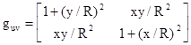
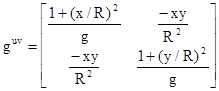
where the components of the "metric tensor" are |
|
|
|
|
|
|
|
Note that we can measure ds for any given dx and dy directly on our surface, so the metric components are purely intrinsic properties of the surface. The metric tensor is a symmetric covariant tensor of second order, and can be written in matrix form as |
|
|
|
|
|
|
|
The determinant of this
matrix at the point (x,y) is g = 1 + (r/R)2 where r = |
|
|
|
|
|
|
|
where summation is implied over repeated indices, and δab is defined as the identity matrix |
|
|
|
|
|
|
|
Solving the preceding equation gives the contravariant tensor |
|
|
|
|
|
|
|
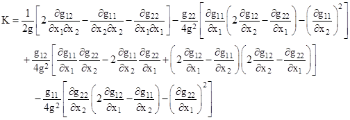
What can we do with this "metric machinery"? Gauss derived the following formula for the curvature K of a surface in terms of the metric tensor and its first and second derivatives. |
|
|
|
|
|
|
|
This is the same K that we defined previously as the product of the two principal curvatures C1 and C2 of the surface at a given point. If we were to construct orthogonal xy coordinates on a plane tangent to this surface at the given point, and then express the perpendicular "height" of the surface away from this plane by an quadratic form f(x,y) = ax2 + bxy + cy2, then we could compute K = C1C2 = 4ac – b2, just as we did previously. Gauss's formula essentially does all that work for us, which is why it is so complicated. (See Note 3.) Substituting the appropriate components into this formula gives |
|
|
|
|
|
|
|
where r2 = x2 + y2. Since the curvature depends only on r, this shows that the lines of constant curvature for this surface are circles when projected onto the xy plane. We can also see that this result agrees with our earlier "extrinsic" derivation, which showed that the curvature at a point on a surface z = ax2 + bxy + cy2 where the xy plane of the orthogonal xyz coordinates is tangent to the surface is simply K = 4ac – b2. In this case our surface is tangent at r = 0 to the xyz coordinates with respect to which the equation of the surface is z = xy/R, so we have a = c = 0 and b = 1/R, so K(0,0) = –1/R2. |
|
|
|
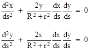
In addition, using the metric tensor, its inverse, and partial derivatives we can now directly compute the "Christoffel symbols", from which we can give explicit parametric equations for the geodesic paths on our surface: |
|
|
|
|
|
|
|
This shows that if either dx/ds or dy/ds equals zero, then the second derivatives of x and y with respect to s must be zero, which means that lines of constant x and lines of constant y are geodesics (as expected, since these are straight lines in space). Of course, given an initial trajectory that is not parallel to either the x or y axis the resulting geodesic path on this surface will be curved, and can be explicitly computed from the above formulas. |
|
|
|
|
|
Notes: |
|
|
|
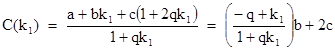
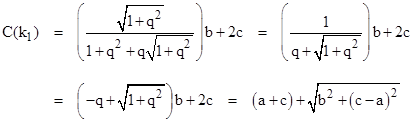
1. Direct substitution of the principal k values into the curvature formula gives a somewhat complicated expression, and it may not be obvious that it reduces to the expression given in the text. To verify the result, recall that we have |
|
|
|
|
|
|
|
where q = (c–a)/b. The roots of the right hand quadratic in k are |
|
|
|
|
|
|
|
To evaluate C(k1), it’s convenient to begin by replacing k2 in the equation for C(k) with 1+2qk1, so we have |
|
|
|
|
|
|
|
Substituting the value of k1 into this equation gives |
|
|
|
|
|
|
|
The similar derivation applies to the other principle curvature if we replace k1 and k2. |
|
|
|
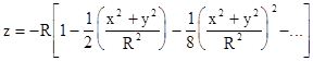
2. To verify this, note that the surface of a sphere of radius R is described by x2 + y2 + z2 = R2, and we can consider a point at the South pole, tangent to a plane of constant z. Then we have |
|
|
|
|
|
|
|
Taking the negative root (for the South Pole), factoring out R, and expanding the radical into a power series in the quantity (x2 + y2) / R2 gives |
|
|
|
|
|
|
|
Without changing the shape of the surface, we can elevate the sphere so the South pole is just tangent to the xy plane at the origin by adding R to all the z values. Omitting all powers of x and y above the 2nd, this gives the quadratic equation of the surface at this point |
|
|
|
|
|
|
|
Thus we have z = ax2 + bxy + cx2 where |
|
|
|
|
|
|
|
from which we compute the curvature of the surface |
|
|
|
|
|
as expected. |
|
|
|
3. To show the economy of Gauss's general formula for the curvature invariant K in terms of the metric tensor components, and to demonstrate that it represents nothing but 4ac – b2 where a,b,c are the coefficients of the quadratic expression for the (embedded) surface with respect to orthogonal coordinates on the tangent plane, we will derive K from the extrinsic point of view for the surface z = xy/R. Obviously the point at the origin is already tangent to the xy plane, so we immediately have a = 0, b = 1/R, c = 0 for that point, which gives K = 4ac – b2 = –1/R2, which agrees with Gauss's formula at the origin (i.e., with x = y = r = 0). More generally, to find the curvature at an arbitrary point (x0,y0) on the surface we re-write the equation of the surface so that this point is at the origin, i.e., z = (x–x0)(y–y0)/R. Then we lower the surface by subtracting x0y0/R from each z value, leading to the equation |
|
|
|
|
|
|
|
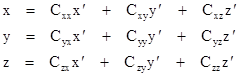
We want to determine the curvature of this surface at the origin. However, the xy plane is not tangent to the surface at this point, as is clear from the non-zero values of ∂z/∂x and ∂y/∂x. We need to rotate our entire xyz coordinate system about the origin so as to make the surface tangent to the xy plane. To do this we can apply the general three-dimensional rotation |
|
|
|
|
|
|
|
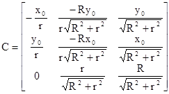
If we substitute these expressions for x,y,z into the preceding equation, we get a general 2nd degree surface in x′y′z′ space, and the condition of tangency requires that the coefficients of x' and y' vanish. One rotation matrix that accomplishes this is |
|
|
|
|
|
|
|
where r = |
|
|
|
|
|
|
|
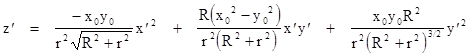
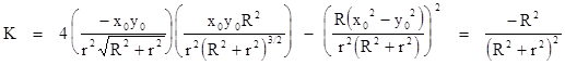
Now we can compute the Gaussian curvature K of this surface as simply the product of the principal curvatures, which for the surface z = ax2 + bxy + cy2 is simply 4ac–b2. Thus we have |
|
|
|
|
|
|
|
which agrees with the result of applying the Gaussian formula to the metric of this surface. |
|
|