Frequency Response and Numerator Dynamics

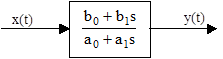
One of the most common representations of dynamic coupling between two variables x and y is the "lead-lag" transfer function, which is based on the ordinary first-order differential equation

where a₀, a₁, b₀, and b₁ are constants. This coupling is symmetrical, so there is no implicit directionality, i.e., we aren't required to regard either x or y as the independent variable and the other as the dependent variable. However, in most applications we are given one of these variables as a function of time, and we use the relation to infer the response of the other variable. To assess the "frequency response" of this transfer function we suppose that the x variable is given by a pure sinusoidal function x(t) = Asin(ωt) for some constants A and ω. Eventually the y variable will fall into an oscillating response, which we presume is also sinusoidal of the same frequency, although the amplitude and phase may be different. Thus we seek a solution of the form

y(t) = Bsin(ωt - θ)

for some constants B and θ. Accordingly the derivatives of x(t) and y(t) are

Substituting for x, y, and their derivatives into the original differential equation gives

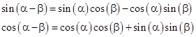
We can expand the sine and cosine functions on the left hand side by means of the trigonometric identities

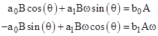
and then set the coefficients of sin(ωt) and cos(ωt) to zero. This yields two equations

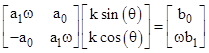
Letting k denote the amplitude ratio k = B/A, we can write these equations in matrix form as

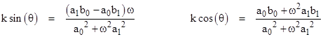
As a result we have

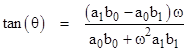
Dividing one by the other gives

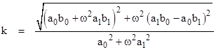
To determine k, recall that if tan(θ) = z then sin(θ) = z/(1+z²)^1/2. Making this substitution in the equation for k sin(θ) gives

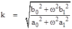
The quantity inside the square root sign is the general form of the Fibonacci identity for the composition of binary forms. Thus if we expand this quantity we find that it factors into the product of two sums of squares, i.e.,

Hence the expression for k simplifies to

The expressions for tan(θ) and k reveal the directional symmetry of the basic transfer function, because exchanging the "a" and "b" coefficients simply reverses the sign of the phase difference θ, and gives the reciprocal of the amplitude ratio k.

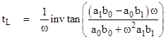
If we define the "time lag" t_L of the transfer function as the phase lag θ divided by the angular frequency ω, it follows that the time lag is given by

For sufficiently small angular frequencies the input function and the output response both approach simple linear "ramps", and since invtan(z) goes to z as z approaches zero, we see that the time lag goes to

The ratios a₁/a₀ and b₁/b₀ are often called, respectively, the lag and lead time constants of the transfer function, so the "time lag" of the response to a steady ramp input equals the lag time constant minus the lead time constant. Notice that it is perfectly possible for the lead time constant to be greater than the lag time constant, in which case the "time lag" of the transfer function is negative. In general, for any frequency input (not just linear ramps), the phase lag is negative if b₁/b₀ exceeds a₁/a₀. Needless to say, this does not imply that the transfer function somehow reads the future, nor that the input signal is traveling backwards in time. The reason the output appears to anticipate the input is simply that the forcing function (the right hand side of the original transfer function) contains not only the input signal x(t) but also its derivative dx/dt (assuming b₁ is non-zero), whose phase is π/2 ahead. (Recall that the derivative of the sine is the cosine.) Hence a linear combination of x and its derivative yields a net forcing function with an advanced phase.

Thus the effective forcing function at any given instant does not reflect the future of x, it represents the current x and the current dx/dt. It just so happens that if the sinusoidal wave pattern continues unchanged, the value of x will subsequently progress through the phase that was "predicted" by the combination of the previous x and dx/dt signals, making it appear as though the output predicted the input. However, if the x signal abruptly changes the pattern at some instant, the change will not be foreseen by the output. Any such change will only reach the output after it has appeared at the input and worked its way through the transfer function. One way of thinking about this is to remember that the basic transfer function is directionally symmetrical, and the "output signal" y(t) could just as well be regarded as the input signal, driving the "response" of x(t) and its derivative.

We sometimes refer to "numerator dynamics" as the cause of negative time lags, because the b₁ coefficient appears in the numerator of the basic dynamic relationship when represented as a transfer function with x(t) as an independent "input" signal, as shown below.

The ability of symmetrical dynamic relations to extrapolate periodic input oscillations so that the output has the same phase as (or may even lead) the input accounts for many interesting effects in physics. For example, in electrodynamics the electrostatic force exerted on a uniformly moving test particle by a "stationary" charge always points directly toward the source, because the field is spherically symmetrical about the source. However, since the test particle is moving uniformly we can also regard it as "stationary", in which case the source charge is moving uniformly. Nevertheless, the force exerted on the test particle always points directly toward the source at the present instant. This may seem surprising at first, because we know changes in the field propagate at the speed of light, rather than instantaneously. How does the test particle "know" where the source is at the present instant, if it can only be influenced by the source at some finite time in the past, allowing for the finite speed of propagation of the field? The answer, again, is numerator dynamics. The electromagnetic force function depends not only on the source's relative position, but also on the derivative of the position (i.e., the velocity). The net effect is to cancel out any phase shift, but of course this applies only as long as the source and the test particle continue to move uniformly. If either of them is accelerated, the "knowledge" of this propagates from one to the other at the speed of light.

An even more impressive example of the phase-lag cancellation effects of numerator dynamics involves the "force of gravity" on a massive test particle orbiting a much more massive source of gravity, such as the Earth orbiting the Sun. In the case of Einstein's gravitational field equations the "numerator dynamics" cancel out not only the first-order phase effects (like the uniform velocity effect in electromagnetism) but also the second-order phase effects, so that the "force of gravity" on an orbiting points directly at the gravitating source at the present instant, even though the source (e.g., the Sun) is actually undergoing non-uniform motion. In the two-body problem, both objects actually orbit around the common center of mass, so the Sun (for example) actually proceeds in a circle, but the "force of gravity" exerted on the Earth effectively anticipates this motion.

The reason the phase cancellation extends one order higher for gravity than for electromagnetism is the same reason that Maxwell's equations predict dipole waves, whereas Einstein's equations only support quadrupole (or higher) waves. Waves will necessarily appear in the same order at which phase cancellation no longer applies. For electrically charged particles we can generate waves by any kind of acceleration, but this is because electromagnetism exists within the spacetime metric provided by the field equations. In contrast, we can't produce gravitational waves by the simplest kind of "acceleration" of a mass, because there is no background reference to unambiguously define dipole acceleration. The Einstein field equations have an extra degree of freedom (so to speak) that prevents simple dipole acceleration from having any "traction". It is necessary to apply quadrupole acceleration, so that the two dipoles can act on each other to yield a propagating effect.

In view of this, we expect that a two-body system such as the Sun and the Earth, which produces almost no gravitational radiation (according to general relativity) should have numerator dynamic effects in the gravitational field that give nearly perfect phase-lag cancellation, and therefore the Earth's gravitational acceleration should always point directly toward the Sun's position at the present instant, rather than (say) the Sun's position eight minutes ago. Of course, if something outside this two-body system (such as a passing star) were to upset the Sun's pattern of motion, the effect of such a disturbance would propagate at the speed of light. The important point to realize is that the fact that the Earth's gravitational acceleration always points directly at the Sun's present position does not imply that the "force of gravity" is transmitted instantaneously. It merely implies that there are velocity and acceleration terms in the transfer function (i.e., numerator dynamics) that effectively cancel out the phase lag in a simple periodic pattern of motion.

Return to MathPages Main Menu