The Filter Of Observation

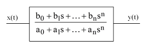
The correspondence between continuous and discrete transfer functions in signal filtering involves many of the same issues that arise in the consideration of measurement in quantum mechanics. Let x(t) denote a real physical variable regarded as a continuous function of time. We might attempt to construct a model dealing directly with x(t), but since any transfer of information must itself constitute a physical effect (i.e., we cannot observe x without physically interacting with it) we should base our model on a dynamic coupling to x(t) rather than on x(t) itself. A typical continuous-time dynamic coupling (i.e., filter) can be expressed schematically as a transfer function

where 's' denotes the differential operator. Here x(t) is the subject physical variable and y(t) is our observation of x(t) achieved via the coupling. This transfer function simply signifies that x(t) and y(t) are related according to the ordinary differential

It's worth noting that this coupling is symmetrical; neither x(t) nor y(t) must necessarily be regarded as the independent or dependent variable. The transfer function simply establishes a coupling between the two; y(t) is our observation of the system variable x(t), and conversely x(t) is the system's "observation" of our variable y(t).

Of course, this coupling by itself does not uniquely determine either x(t) or y(t). Each of these variables is subject to its own system constraints. By examining y(t) we hope to discern the constraints on x(t), from which we will infer something about the system of which x is a part. At the same time the constraints we impose on y(t) on our side of the coupling have an influence on x(t) and the system being observed.

The situation becomes more interesting when we attempt to translate such a coupling into the discrete-time domain (as, for example, when we model a continuous filter on a digital computer). In this case we can deal explicitly only with the values of the variables at discrete time intervals, i.e., we have only the values x(kτ) and y(kτ) where k = ... -1, 0, 1, 2 … and τ is a constant time increment.

How do we translate the continuous transfer function into an equivalent coupling between the discrete-time values of x and y? There is no single discrete-time formula that will match the continuous relation for all possible signals x(t) and y(t) because the discrete-time model has no knowledge of the behavior of the signals at frequencies greater than 2π/τ. However, there are two specific translations that are, in different respects, optimum. One of these can be identified with "observed interactions" while the other can be identified with "unobserved interactions".

Suppose we intend to make a measurement of the variable x(t) associated with a particular system. For this purpose we design an interaction between x(t) and our local variable y(t) such that y(t) is as free of constraints (on our side of the coupling) as possible. In this context we can essentially treat x(t) as an independent variable and y(t) as the dependent variable (i.e., entirely dependent on x(t)). Now, given a sequence of discrete values x(0), x(τ), x(2τ),...x(nτ) we still need to assume something about the form of the continuous variable x(t) in order to solve equation (1) for y. Of all the possible continuous functions, one could argue that the "most probable" is the unique nth degree polynomial that passes through the given values of x(kτ). On that basis we can define the unique discrete-time recurrence relation corresponding to (1) with matched homogeneous response for y(t).

In contrast, consider an interaction in which x(t) and y(t) are symmetrical with respect to our state of knowledge, i.e., neither of them is regarded as “given”. In this context the optimum discrete-time recurrence is given by matching the homogeneous response of (1) "in both directions", i.e., for both x(t) and y(t). The resulting discrete-time recurrence is symmetrical and reversible.

Letting X and Y denote the column vectors with the components x(kτ) and y(kτ) respectively for k = 0, 1, ..., n, the general form of the discrete-time recurrence is

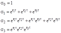
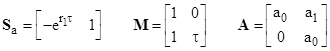
where S_a and G are constant row vectors. The components of S_a are the elementary symmetric functions (with alternating signs) of the exponentials of the roots of the characteristic equation of the left side of (1). For example, with a third order differential equation let r₁, r₂, r₃ denote the roots of the characteristic polynomial

The symmetric functions of the exponentials are

and we define the row vector S_a as

For future use, we define the row vector S_b in terms of the characteristic roots of the right side of (1) in the similar way.

The components of G depend on which of the two contexts is assumed. For a "measurement coupling" when y(t) is treated as a purely dependent variable we have

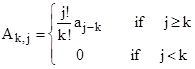
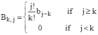
where A, B, and M are square matrices defined by

On the other hand, if we treat x(t) and y(t) symmetrically (i.e., a non-measurement coupling) we have

where the summations in the numerator and denominator represent the sums of the components of S_a and S_b respectively. The G vectors given by (2) and (3) converge to each other in the limit as τ goes to zero.

One interesting aspect of these two forms of filters is that when we impose a "direction" on the transfer of information by determining one of the two sides of the equation, the resulting "most probable" transfer is irreversible, whereas if we allow the interaction to exist "unobserved" the most probable transfer is perfectly time-symmetric and reversible. This seemingly paradoxical situation arises only in the discrete-time case when the elementary increment of time τ is non-zero.

Equating the two expressions for G given by (2) and (3), and re-arranging terms, we get

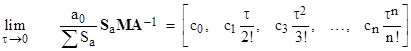
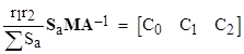
Since we can choose the a and b coefficients independently, we see that the expression on the left side approaches the same row vector as τ goes to zero, regardless of the components of A. The lowest order non-zero components of this n+1 dimensional row vector are

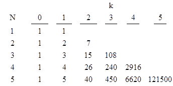
where the coefficients c_k are as shown below

These coefficients can be generated using Eulerian numbers, and are closely related to the generalized Bernoulli numbers. To illustrate, consider first the simple case n=1, with the homogeneous equation

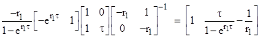
The has the characteristic equation a₀ + a₁r = 0, with the root r₁ = –a₀/a₁. In this case we have the matrices

It’s convenient to express the coefficients in terms of the roots, and by scaling we can set a_n = 1, so we have a₀ = –r₁, and hence

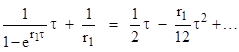
Expanding the second component to a series in τ, we have

This confirms that, to the lowest order, the second component is just (1)τ/2!, in agreement with the table.

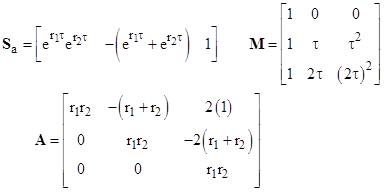
Likewise for a second-order equation (scaled so a₂ = 1) we have the matrices

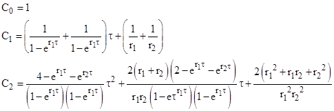
From these, and remembering that a₀ = r₁r₂, we can compute

where

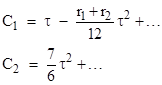
Expanding the expressions for C₁ and C₂ into series in τ, we get

which again confirms the coefficients in the table for the lowest order non-zero terms.

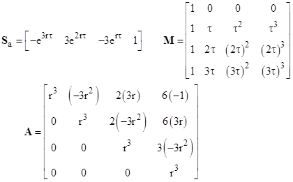
For higher-order equations (with three or more characteristic roots) the full calculations become very complicated, but we can simplify by considering some special cases. For example, suppose all n roots are identical. (Admittedly these “repeated roots” lead to different forms for the general solutions, but that doesn’t upset our results.) On this basis the computations are simplified. For a third-order equation with three identical characteristic roots r, we have the matrices

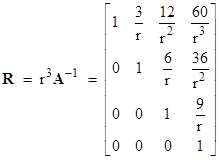
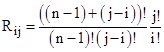
Defining R as rⁿ times the inverse of the A matrix, we have

The non-zero coefficients (j ≥ i) are

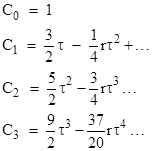
With these matrices for the case n=3 we can compute

and expand the coefficients in powers of τ to give

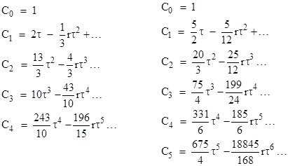
In the same way we find that the limiting vectors for n=4 and n=5 are

Another class of equations that can be analyzed explicitly is those with cyclotomic characteristic polynomials, i.e., of the form xⁿ – 1 = 0. For these equations the only non-zero coefficients of the equation are a_n = 1 and a₀ = –1. With n=1 the single root is r = 1, and we must consider each term in the series expansion of the exponential

On the other hand, for n=2 we have the two roots r₁ = 1 and r₂ = –1, which implies that all the odd terms in the expansion of the first symmetric function cancel out, so the only non-zero terms are the even terms

To get the lowest order result we could almost neglect the fourth degree term, but not quite, because it contributes (1/6)τ² to the value of C₂ = (7/6)τ². However, for all odd values of n greater than 2 only the lowest order correction is relevant. For example, with n=3 we have the three cube roots of 1, and sums of the kth powers of these roots vanish identically unless k is a multiple of 3, in which case the sum of 3. Hence the lowest order correction is proportional to τ³, and the next non-zero correction is proportional to τ⁶, which is too small to be relevant. So, for the cyclotomic case with n=3 it is sufficient to approximate the S_a row vector by

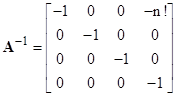
The second symmetric function of the exponential has a negative correction because the coefficients of the first and second degree corrections are zero and the coefficient of the third degree correction has quantities such as r₁³/3 + r₁²r₂/2 + r₁²r₃2/2 which equals –r₁³/6. Noting that the inverse of the A matrix for this cyclotomic equation is

and that a₀ = –1 and that the sum of the components of S_a is just –τ³, we can compute

in agreement with the previous results.

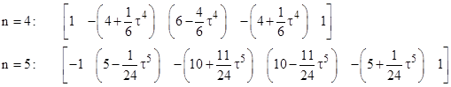
The truncated S_a vectors for the next two orders of cyclotomic equations are listed below.

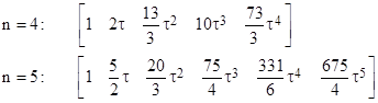
The numerators of the corrections to the basic binomial components are the Eulerian numbers, such as (1, 11, 11, 1) for n=5. With these we compute the limiting S_aMA^–1/τⁿ vectors

These results agree with the previous coefficients (i.e., those based on equal roots) except for the highest coefficient 73/3 in the case n=4. The previous results were 243/10, which differs by 1/30. In general, if we define the Bernoulli numbers by the generating function

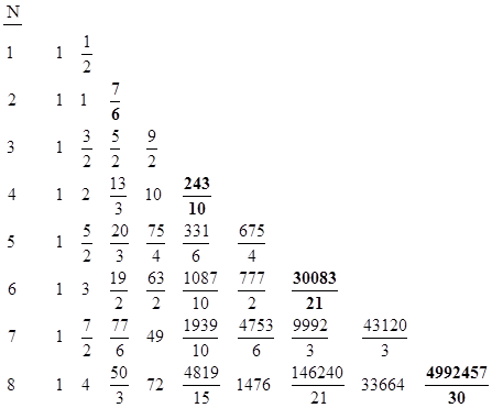
then we find that our limiting coefficients based on the truncated cyclotomic case differ from the true coefficients (such as given by the equal root analysis) at order N by the fact that the highest order coefficients differ by the amount B_N. The Bernoulli numbers vanish for odd N greater than 1, so this affects only the limiting coefficients for even values of N. Taking this into account, the limiting coefficients up to N=8 are summarized in the table below.

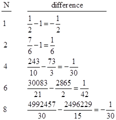
The differences between the highest coefficients for the truncated cyclotomic method and the equal root method for even N are shown below:

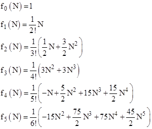
The columns of the limiting coefficient table are produced by the polynomials

and so on. Note that f_k(0)=0 and f_k(1)=k!. Each f_k(N) is the coefficient of τ^k, and if we partition a unit interval of time into N segments we have τ = 1/N. It follows that each f_k(N)τ^k asymptotically approaches the coefficient of N^k, and we see that these asymptotic values are 1/2^k.

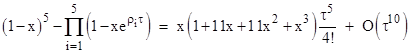
As an aside, this provides a kind of generating function for the Eulerian numbers. For example, we have

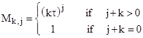
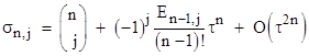
where the ρ_i are the 5th roots of unity. In general, if σ_n,j denotes the jth elementary symmetric function of the exponentials of ρ_iτ where ρ_i are the nth roots of unity, then

for j = 1 to n–1, with symmetrical indices for the Eulerian numbers such that the top “1” is E_1,1.

Return to MathPages Main Menu