Integrating Factors

The solution of a homogeneous first-order linear differential equation of the form

where a(x) and b(x) are known functions of x, is easy to find by direction integration. Multiplying through by dx, dividing through by a(x)y, and re-arranging the terms gives

Integrating both sides, we have

where K is an arbitrary constant of integration. Taking the exponential of both sides gives the solution

However, this simple method of solution works only because the original differential equation was homogeneous, i.e., the right hand side of the original equation was zero. The solution is slightly more complicated if the right hand side is not zero. Consider an ordinary first-order differential equation of the form

where a(x), b(x), and c(x) are known functions of x. Notice that if b(x) happens to be the derivative of a(x), then the left hand side is the derivative of the product a(x)y. In that special case we have

so we can integrate both sides to give

where K is an arbitrary constant of integration. Solving for y gives the result

Of course, this works only in the special case that the coefficient of y in the original differential equation (i.e., the function b(x)) happens to be the derivative of the coefficient of dy/dx (i.e., the function a(x)), which is not generally the case. However, it may be possible to bring the original differential equation into this special form by simply multiplying through by another function f(x). Such a function is called an integrating factor. We have

and we want to choose f(x) so that f(x)b(x) is the derivative of f(x)a(x). Thus we impose the condition

Re-arranging terms, this condition can be written in the form

Notice that this is a homogeneous equation in f(x). If we let a′-b denote the quantity inside the square brackets (i.e., the coefficient of f(x)), then we already know (from above) that the solution of this equation is

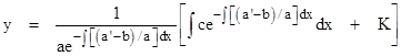
for some arbitrary constant k. With this, the solution of the non-homogeneous equation (1) is given by (2) if we replace a(x) with f(x)a(x) and replace c(x) with f(x)c(x). Notice that the constant factor e^k appears in both of these terms, so it cancels out of the first distributed term in (2), and can be absorbed into the arbitrary constant K in the second term. Thus we can omit the factor e^k without loss of generality, and overall solution can be written in the form

Naturally if b(x) equals the derivative of a(x), this reduces to equation (2).

A simpler way of expressing the general solution is to begin by dividing through the original differential equation (1) by a(x), so that the leading coefficient equals 1. Then we have new functions b(x) and c(x) (equal to b/a and c/a in terms of the original functions) such that

Taking a(x) = 1 and a'(x) = 0 in the preceding expression we have the familiar result

It is also possible to use integrating factors to solve certain non-linear differential equations. Consider an equation of the form

where A and B are arbitrary (differentiable) functions of x and y. Obviously equation (1) is a special case of this, given by setting A(x,y) = a(x) and B(x,y) = b(x)y - c(x). Multiplying through by the differential dx, we have

Notice that if there exists a function ϕ(x,y) such that

then the preceding equation can be written in the form

We recognize the left hand side as the total differential dϕ, so it follows (in this case) that dϕ = 0, which means that ϕ(x,y) is invariant, i.e.,

for some constant C. For example, consider the equation

This represents a total differential equation (also called an exact differential equation), because there exists a function ϕ(x,y) whose partial derivatives equal the coefficients in parentheses. Specifically, setting ϕ(x,y) = (1/2)x² + xy + (3/2)y² we have

Therefore the differential equation is equivalent to the algebraic condition that ϕ(x,y) is invariant, i.e., the solution is of the form

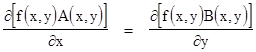
It's easy to recognize when a differential equation is "total" (exact) if we recall that partial differentiation is commutative, i.e., for any function ϕ(x,y) we have

An equation of the form (3) is total if and only if the partials of a function ϕ(x,y) with respect to y and x respectively are equal to the coefficient functions A(x,y) and B(x,y), and from the commutative property of partial differentiation we see that this will be true if and only if the partials of A and B with respect to x and y respectively are equal. Hence the necessary and condition for (3) to be a total differential equation is

In cases when this does not hold, it is still sometimes possible to apply an integrating factor so that the resulting equation is total. In other words, even if the above equality is not satisfied, there may exist a function f(x,y) such that

in which case we can multiply through equation (3) by f(x,y) to give a total differential equation. Using subscripts to denote partial derivatives, we seek a function f(x,y) such that

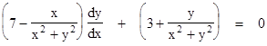
As an example, suppose we wish to solve the equation

In this case we have A(x,y) = 7x² - x + 7y² and B(x,y) = 3x² + y + 3y², and so the equation does not correspond to a total derivative, because A_x(x,y) = 14x - 1 whereas B_y(x,y) = 1 + 6y. However, if we multiply through the above equation by 1/(x² + y²), the differential equation becomes

which is total, because the partials of the coefficients in parentheses are both equal to (x² - y²)/(x² + y²)². Integrating these coefficients, we find that the they are the partials of the function

and we know the total differential of this function is invariant, so the solution of the differential equation satisfies the condition

where C is an arbitrary constant of integration.

Return to MathPages Main Menu