The Orbit of Triangles

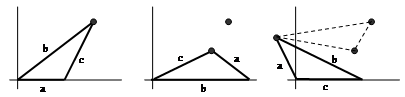
Consider an arbitrary non-equilateral triangle with edge lengths a, b, and c. Place the edge of length a on the segment [0,a] of the x-axis of a Cartesian coordinate system and mark the location of the opposite vertex. Then place the edge of length b on the x-axis at [0,b] mark the location of the opposite vertex. Finally, place the edge of length c on the x-axis at [0,c] and mark the location of the opposite vertex. The three marks constitute a new triangle, with edge lengths a′, b′, and c′.

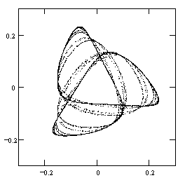
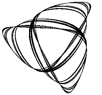
This process can be repeated indefinitely. At each stage it’s convenient to normalize the size of the triangle by magnifying or shrinking it so the perimeter has length 1. The sequence of triangles produced by iteration of this procedure then consists of a sequence of triples {a,b,c} with a + b + c = 1. Taking a,b,c as Cartesian coordinates, each triangular shape can be plotted in three-dimensional space, and the condition a + b + c = 1 implies that all the points fall on a single plane. The attractor of these points is a beautiful closed curve that somewhat resembles a trefoil knot, as shown below.

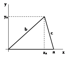
It should be noted that this iteration is sensitive to the choice of permutations for the edge lengths.  In some implementations the constructed triangles degenerate into straight lines, so it’s important to select the right permutation. To make the construction of these points explicit, we begin by describing how to compute the raw vertices of the new triangle from the edge lengths a,b,c of any given triangle. The first vertex is found by placing the edge length “a” on the x axis as shown below.

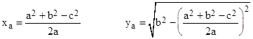
By Pythagoras’ theorem we have

Solving these equations for x_a and y_a, we get

By cyclic permutation of the variables, we also have the coordinates of the other two vertices of the new triangle

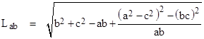
Letting L_ab denote the length of the edge from the vertex at x_a,y_a to the vertex at x_b,y_b, we can now compute

The values of y_a and y_b are defined in terms of square roots, and the above expression contains a term of the form -2y_ay_b, so we might expect the result, when expressed in terms of the original edge lengths a,b,c, to involve a square root inside the square root. However, notice that the y_a and y_b coordinates represent the heights of the original triangle on the respective bases, so we have

where A is the area of the original triangle, and therefore by Heron’s formula

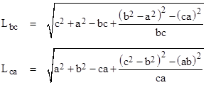
Making use of this fact, we can insert the previous expression for the coordinates and simplify to arrive at the length of the edge of the new triangle

By cyclic permutation of the variables, we arrive at the other two edge lengths

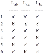
These are the edge lengths of the new triangle (prior to normalization), but we have six choices for how to assign these values to the new set of edge lengths which we will call a′, b′, and c′. These choices are shown below

Choices 1, 3, and 5 each produce the "trefoil attractor". If we choose 2 or 4 the resulting iteration converges on a 3-cycle of segments of length {0.309016, 0.190983, 0.500000}, which corresponds to a degenerate triangle with three co-linear vertices, one of which cuts the segment connecting the other two in the "golden proportion" 1.61803.... If we choose permutation 6 the sequence converges on a 1-cycle of this same "golden" line segment.

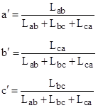
Taking choice 1, and normalizing the edge lengths, we have the iteration

Viewing these values as the Cartesian coordinates of a point in three-dimensional space, and noting that a′ + b′ + c′ = 1, we see that the points all fall in a single plane. We can transform from a,b,c to coordinates in a single plane simply by rotating the points {a,b,c} first about the b axis using the transformation X = Aa - Bc, Y = b, Z = Ba + Ac with A² + B² = 1, and then rotating about the X axis by the transformation x = X, y = αY – βZ, z = βY + αz with α² + β² = 1. The composition of these is

We want all the points to have the same value of z for any a,b,c, so we must have β = αA = αB. Thus we have β² = α²A² and β² = α²B², from which we get 2β² = α², and hence 3β² = 1 and 3α² = 2. It follows that A² = B² = 1/2. Taking the positive roots for all these coefficients, we have the total transformation

This gives the "trefoil attractor" described above. An enlarged image of this locus is shown below.

If we exand the view of this locus, we find that each of the curves actually splits into multiple distinct curves, each of which splits into multiple curves on even closer examination, and so on.

Return to MathPages Main Menu