Potential Flow and D'Alembert's Paradox

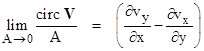
For a vector function V(x,y,z) in space, let v_x, v_y, and v_z denote the components of V. The circulation of the vector field V around any simple closed path S is defined as the integral of the tangential component of V around that path (in the "right-handed" direction). If the path is defined parametrically as a function of the path length parameter s by equations for x_p(s), y_p(s), z_p(s), then the unit tangent vector as a function of s is

This is automatically a unit vector because (ds)² = (dx_p)² + (dy_p)² + (dz_p)² by definition. Since we know the components of V as a function of x,y,z, and we know the values of x_p,y_p,z_p as a function of s around the closed path, we can express the components of V as functions of s on the path. Thus we have the vector functions V(s) and p(s) for points on the path. Recall that the dot product of two vectors is a scalar whose magnitude equals the product of the magnitudes of the arguments times the cosine of the angle between them. Thus the dot product of V and p is the projection of V along the tangent direction, and so the circulation of V around the path S is simply the integral

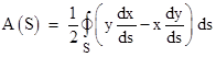
If the path S is planar, we can also determine the enclosed area by means of a simple integration. For example, if the path lies entirely in the xy plane, the area is given by

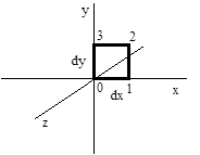
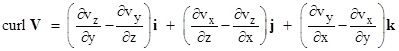
At every point in space we can define "curl V" as a vector whose components in each of the three principle directions equal the circulation around a closed path, in the plane normal to that direction, divided by the area enclosed by the path in the limit as the area goes to zero. Without loss of generality we can assume square paths, so the z component of the curl of V can be expressed as the limit of the circulation around a square path in a plane parallel to the xy plane.

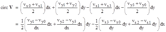
Since we are going to take the limit as the area goes to zero, and all the partial derivatives of the vector field are finite (by assumption), we can choose a small enough square so that the field is planar over this region. In other words, the change in the components of V from 0 to 1 is the same as the change from 2 to 3, and the change from 1 to 2 is the same as from 0 to 3. Also, the components vary linearly along each edge. In addition, notice that the projection of V along each edge of the square is just the respective component of V. Therefore, the circulation around this square path is

Since the changes in the components along opposite edges are equal, this reduces to

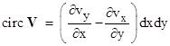
Obviously the area enclosed by this path is simply dxdy, so the limit of the circulation in the plane normal to the z direction as the area of the path goes to zero is

(It can be shown that the limiting circulations are independent of the shape of the path.) Hence this is the z component of the curl of V. In the same way we can evaluate the limiting circulation for closed paths around this same point in planes normal to the y and x directions to give the y and x components of the curl.  Letting i,j,k denote basis vectors in the x,y,z directions respectively, the curl can be written as

In fluid mechanics if the vector field V represents the velocity of the fluid at each point, then curl V is called the vorticity of the fluid at that point. The vorticity is just twice the angular velocity vector.

If the vorticity of a flowing fluid is everywhere zero, then the flow is said to be irrotational. Kelvin showed that vorticity is conserved in an ideal non-viscous incompressible fluid, so if the fluid is irrotational at any instant, it remains irrotational thereafter. This is important because we often imagine a large reservoir of essentially static or uniformly flowing (and therefore irrotational) fluid as the upstream boundary condition of a problem, and we can therefore assume the flow is irrotational throughout the process. Of course, the assumption of zero viscosity, and the absence of boundary layer effects, is never perfectly correct, and it's obviously possible to introduce or remove vorticity due to real-world boundary layer effects. Nevertheless, in a large class of realistic situations the assumption of irrotational flow is valid.

Under these conditions there exists a scalar field ϕ(x,y,z) such that the fluid velocity vector is the negative gradient of ϕ. In other words, letting v_x, v_y, v_z denote the components of the fluid velocity in the principle directions, we have

The scalar ϕ is called the velocity potential. To prove that such a scalar function ϕ exists for irrotational flow, recall that partial differentiation is commutative on a flat manifold, which means that for any scalar field ϕ we have (for example)

Substituting –v_x for ∂ϕ/∂x and –v_y for ∂ϕ/∂x, we have

which represents the vanishing of the z component of the vorticity. Likewise the vanishing of the other vorticity components is equivalent to the commutation of partial differentiation with respect to the other two pairs of coordinates.

For a continuous fluid medium we have the continuity condition

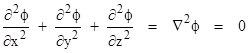
where ρ is the fluid density. For an incompressible fluid the density is a constant, so the continuity condition reduces to simply the vanishing of the divergence, i.e., ∇×V = 0. Inserting the expressions for the components of V in terms of the potential, this gives Laplace's equation

Using this equation, together with appropriate boundary conditions, we can solve for the potential function throughout the flow field, and this yields the streamlines as well, since they are everywhere normal to the equi-potential surfaces. Also, given the velocity of the fluid at each point, we can immediately compute the static pressure as well, and we can integrate this pressure over any surface to find the net force on that surface. Of course, this is all based on the neglect of boundary layers, which can have some surprising consequences as we'll see below.

For a relatively simple example, consider the flow of an ideal incompressible irrotational fluid past a stationary sphere. Letting U denote the free-stream velocity of the fluid, it's clear that the potential field is axially symmetrical about the axis through the sphere parallel to the direction of flow, so we need only specify the potential ϕ as a function of the polar coordinates r (the distance from the sphere's center) and θ (the angle from the direction of flow. Laplace's equation reduces to

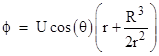
For flow past a sphere we require that the radial component of the flow velocity is zero at the surface of the sphere. (Notice that we do not require the tangential velocity to vanish at the surface, because we are assuming perfectly inviscid, i.e., frictionless, flow.) If the radius of the sphere is R, the general solution for the potential field is

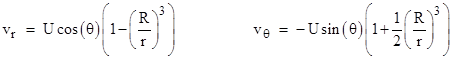
so the components of the flow velocity are

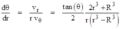
Since v_r = ∂ϕ/∂r and v_θ = (1/r)∂ϕ/∂θ, the streamlines must satisfy the condition

This leads to the integral equation

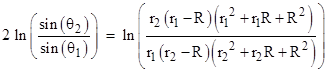
Carrying out the integration gives

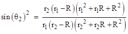
Taking the exponential of both sides and setting θ₁ = π/2 and r₁ equal to the closest approach of the streamline to the sphere, we have

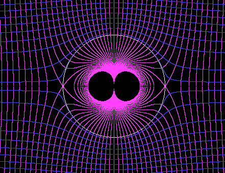
So, for any given r₁ we can compute sin(θ₂) as a function of r₂, and from this we also have cos(θ₂), so we can compute the streamlines as the locus of points with x = r₂ cos(θ₂) and y = r₂ sin(θ₂). A plot of the equi-potential lines and streamlines for the flow past a sphere is shown below.

Notice that there is no boundary layer in this model, so the flow velocity does not go to zero at the surface of the sphere. Consequently the velocity field is symmetrical on the upstream and downstream sides of the sphere. This means the total momentum of the flow is unchanged, so the flow cannot have imparted any momentum to the sphere. Thus the net force exerted by the fluid on the sphere is zero. This can also be seen by noting that since the velocities are symmetrical on the upstream and downstream sides, so are the pressures (using Bernoulli's formula (1/2)ρv² + p₀ = constant to give the static pressure as a function of the flow velocity). Jean Le Rond d'Alembert (1717-1783) performed a series of experiments to measure the drag on a sphere in a flowing fluid, and on the basis of the potential flow analysis he expected that the force would approach zero as the viscosity of the fluid approached zero. However, this was not the case. The net force seemed to converge on a non-zero value as the viscosity approached zero. Hence the vanishing of the net force in the potential flow analysis is known as D'Alembert's Paradox.

Interestingly, this is really just another form of the well-known "limit paradox" in elementary calculus, a paradox that is also historically associated with D'Alembert. The resolution becomes clear when we realize that any non-zero viscosity, no matter how small, will result in a boundary layer that forces the tangential flow velocity to vanish at the surface of the sphere. As we lower the viscosity, the thickness of the boundary layer is reduced, but the flow velocity still drops to zero across that layer (the "no-slip" condition), and the results of this boundary layer, with its vorticity, mixing, and possible separation, lead to losses in the momentum of the flowing fluid and the transference of momentum to the sphere, i.e., to a net unbalanced force, roughly proportional to the velocity of the freestream flow (for relatively slow flow velocities). The correspondence with the limit paradox from calculus is obvious, i.e., the limiting condition of a sequence need not possess all the properties possessed by all the members of the sequence.

Incidentally, D'Alembert was given the name Jean Le Rond because as an infant he was found abandoned on the steps of the St. Jean Baptiste le Rond church. He was placed in the care of foster parents, to whom he remained loyal all his life, even after it was discovered that his natural mother was an aristocratic lady, Madame de Tencin, and his natural father was the artillery general Chevalier Destouches. D'Alembert became famous as a mathematician and scientist, notable for his development of partial differential equations, particularly the basic wave equation ∂²h/∂t² – ∂²h/∂x² = 0. During the years from 1751 to 1772 he collaborated with Denis Diderot on the famous "Encyclopedia", to which he contributed the preface and most of the articles on science and mathematics.

Return to MathPages Main Menu