Appendix B:  Nth Order Recurrence Formulas

In Sections 2 and 3 the optimum recurrence formulas for first and second order response were derived based on the assumption that the input function x(t) was the first or second-degree polynomial (respectively) that passes through the given discrete values of x(t). In this appendix we generalize this method to Nth order response.

Let x(t) and y(t) denote continuous functions of time, related according to the Nth order differential equation

where the coefficients a_k and b_k are constants, and we stipulate the a_N, a₀, and b_N are non-zero. We will denote by r₁, r₂,..., r_N the roots of the characteristic polynomial

of the left hand side of this differential equation.

First, consider the homogeneous case, i.e., suppose that x(t) is identically zero, so we set the left side of equation (1) equal to zero. From the fact that d(e^rt)/dt equals re^rt it follows that y(t) = Ke^rt satisfies this homogeneous equation for any constant K and any r that is a root of the characteristic polynomial. As a result, the general homogeneous solution is of the form

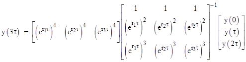
where the K_j are arbitrary constants. (We neglect the complication of repeated roots, because this turns out not to affect the form of the discrete recurrence solutions.) Given the values of y(t) at N evenly-spaced discrete times t = 0, τ, 2τ, …, (N–1)τ, we can solve for the constants K_j, and we can then compute the value of y(Nτ). For example, with N=3 we have

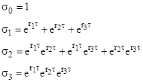
Carrying out the matrix inverse and multiplication, this gives

where

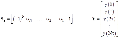
In general, the coefficients of the recurrence for the homogeneous response are the elementary symmetric functions (with alternating signs) of the exponentials of the N quantities r_jτ where r_j are the N characteristic roots and τ is the time increment. For convenience we define the row and column vectors

Since the equation is invariant under time translation, we can set the t=0 at any time, so the Y vector is understood to be representative of any N+1 consecutive samples. In these terms the homogenous recurrence can be written as

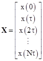
Now we consider the case with non-zero x values, so the right hand side of equation (1) provides a forcing function. We are given a sequence of N+1 evenly spaced discrete values of x(t), which we denote by the column vector

First we note that if the a and b coefficients of corresponding derivatives in equation (1) were the same, we could simply bring the x variable over to the left side, and we would have a homogeneous equation in the variable y–x, so the solution would be S_a(Y – X) = 0. For the more typical case, when the a and b coefficients are different, we will assume that the function x(t) during the interval from t = 0 to Nτ is given by the Nth degree polynomial

where the c_j coefficients are such that this function passes through the N+1 given discrete values. Thus if we define the column vector C and square matrix M by

we have C = M^–1X. We now substitute the polynomial for x(t) into the right side of equation (1) and evaluate the derivatives to give the forcing function

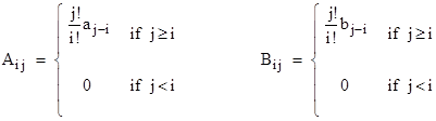
where the components of the square B matrix are defined as shown on the right below

and the indices i and j range from 0 to N. Now, making use of the A matrix defined on the left above, we define a modified X vector, which we will denote as, such that

Thus, if we replace X with  and replace the b coefficients on the right side of equation (1) with the corresponding a coefficients, we will get exactly the same forcing function F(t). In that case, since the coefficients on both sides of (1) are the same, we can bring the modified x values over to the left side and create a homogeneous equation, which (as we’ve seen) has the solution

Solving the previous equation for  and substituting into this equation, we get the result

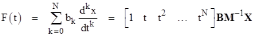
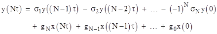
Letting g_i denote the ith element of the row vector given by S_aMA^–1BM^–1, we have the explicit recurrence formula

The values of σ_k are always purely real for real coefficients a_k, even when the roots r₁,r₂,.., r_N are complex. Also, for reasons discussed in Section 2.2.5, the values of σ_k are the exact coefficients of the y samples in the recurrence, regardless of how the x(t) function is interpolated. Only the g_i coefficients would be affected if we changed our assumption as to the form of x(t) (that is, if we identified x(t) with a function different from the Nth order polynomial fit through the given discrete values).

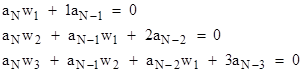
One way of computing σ_k is to algebraically solve the characteristic equation (2) for all the roots r_j, j=1 to N, and then directly compute the symmetric functions of the exponentials. However, finding all the complex roots of an Nth degree polynomial can be computationally laborious and involves numerous special cases. Another approach, one that avoids having to explicitly determine all the roots of the characteristic polynomial, is to use "Newton's sums". For any non-negative integer k, let w_k denote the sum of the kth powers of the roots r₁,r₂,..,r_N. Clearly w₀ = N. The values of w_k for k = 1, 2, ... can be found using the identities

and so on for k < N, and the recurrence

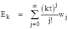
for all k ³ N. Now let E_k denote the sum of the kth powers of the values of , i = 1, 2, .., N. The Taylor series expansion gives

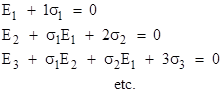
The values of σ_k can now be computed using the identities

Return to Table of Contents