3.  Discrete-Time Simulation of Second-Order Response

3.1  Background

This section treat the discrete-time simulation of any continuous dynamic relationship of the form

where x is the independent variable, y is the dependent variable, t is time, and the coefficients a₁, b₁, a₂, and b₂ are real constants (with a₁ not equal to zero).

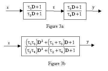
It may appear at first that this type of relationship could be simulated simply by means of two first-order lead/lags in series, as illustrated by Figure 3a, where D denotes the differential operator.  Combining these two (simplistically) gives the second-order transfer function shown in Figure 3b.

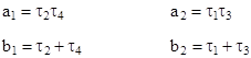
Identifying the coefficients of this function with those of equation (3.1-1) gives

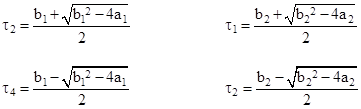
Solving these equations for τ₁ through τ₄, we have

Notice that if 4a₁ is greater than b₁² (meaning that the response is under-damped), then τ₂ and τ₄ are not real numbers.  It follows that first order lead/lags with real coefficients cannot be combined to give an underdamped second-order response.  (This corresponds to the fact that in electrical circuits an oscillating response cannot be produced by any passive arrangement of resistors and capacitors.)  Also, if 4a₂ is greater than b₂², then τ₁ and τ₃ have non-zero imaginary parts.  Thus, unless the function to be simulated is overdamped in both directions (i.e., with either x or y regarded as the dependent variable), it cannot be simulated by a combination of first order functions with real coefficients.  Of course, first-order algorithms can be written to accommodate complex coefficients and variables (noting that the intermediate vairable z in Figure 3 can be complex) and this approach can be generalized to reduce linear differential equations to a set of first-order differential equations, but for embedded code it is often desirable to avoid complex arithmetic.  Furthermore, in discrete-time implementations the combination of two first-order simulation algorithms in series does not give the optimum representation of the corresponding product of continuous first-order functions (see Section 3.3).

The optimum recurrence formula for second-order response is presented in Section 3.2 based on the exact analytical solution of equation (3.1-1) with specific interpolation assumptions for the input variable.

Return to Table of Contents