2.3  Modified First Order Simulation Methods

2.3.1  Simplified Solutions Based on Approximations of e^z

If τ_N and τ_D are constant (and assuming a constant Δt), then the recurrence coefficients A and B are also constant and can be pre-computed off-line using the optimum constant-τ formulas given by equations (2.2.3-4). However, if τ_N and τ_D are variable, the optimum coefficients given by (2.2.4-4) and (2.2.4-5) are rather cumbersome, and require storage of past values of τ_D and τ_N. We have shown that the variable-τ response can be approximated by the constant-τ solution if Δt is small enough, but in this case the A and B coefficients must be recomputed on-line for each interval, and it may be desirable to simplify the computation. Since the most time-consuming aspect of the computation is the exponential in equation (2.2.3-4), the most common approach is to substitute some approximation for this exponential.

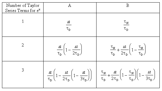
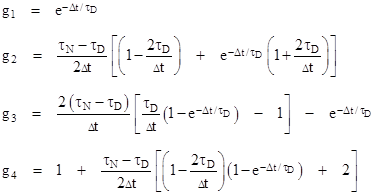
If |Δt/τ_D| is much less than 1, we can substitute the first terms of the Taylor series expansion for e^z into equation (2.2.3-4), which leads to the family of approximate recurrence coefficients presented in Table 1.

Table 1

Many lead/lag algorithms correspond to one of these approximate solutions, or some variation. For example, one simulation program uses an algorithm equivalent to

This corresponds to the lowest order approximation from Table 1, except that B includes a Δt in the numerator. The effect of this Δt is to introduce a bias in the response to non-constant input functions (because B is the coefficient of Δx in the recurrence formula). This bias was not evident during testing because the only evaluation of the algorithm was based on its response to step inputs, during which Δx was always zero except at a step.

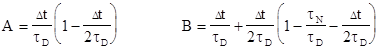
Another example is a commercial embedded software package that uses a lead/lag algorithm with the coefficients

Here, the solution corresponds to the second order approximation from Table 1, except for the –Δt/2τ_D component in the right hand term of B.

It’s interesting to compare all five of the modified B coefficients discussed so far for a particular case. Consider a lead/lag with τ_N/τ_D = 10 and Δt/τ_D = r < 1. The three levels of approximation from Table 1 are

whereas the dynamic simulation algorithm of the first example gives B = 10 + r, and the embedded commercial algorithm of the second example gives B = 10 – (9/2)r – (1/4)r². According to the Taylor series approximation method, the former approximation is wrong in the first order correction for non-vanishing r, while the latter approximation is wrong in the second order. The reason that the designers of these algorithms chose to deviate from the Taylor series approximation as shown here is not known.

Instead of the Taylor series approximation, we could make use of the series expansion of the natural log (see Section 2.2.5). If we take just the first term of this series and make the substitution

we have

Taking the exponential of both sides gives

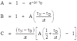
In the range of interest, this is a much more efficient approximation of the exponential than the truncated Taylor series. Substituting this for the exponential in equations

(2.2.3-4) gives the recurrence coefficients

Incidentally, some commercial applications have implemented simple first-order lags which compute y_c based only on x_c and y_p. Since they do not store the past value of x, they effectively assume x_p = x_c. With this assumption the value of B is unimportant, because it is the coefficient of x_c – x_p which vanishes. Hence we’re only interested in the A coefficient, which these applications take to be A = Δt/(τ_D + Δt). Clearly the optimum representation of a first-order lag to this level of approximation would be with A = Δt/(τ_D + Δt/2), as can be seen from the preceding formula. It is not known why the application designers chose to neglect the factor of 1/2 on Δt in the denominator. This makes the effective time constant of the algorithm equal to τ_D + Δt/2. Typically Δt is about 1/4 of τ_D, so this represents up to 25% error in the time constant.

2.3.2  Finite Differences and Bilinear Substitution

The most direct approach to determining an approximate recurrence formula for a differential equation of the form

is to substitute simple finite differences for the differentials about the nearest convenient point. The derivative of the function y(t) at the point half-way between the past and current instants can be approximated by

The value of the function y(t) at this point is approximately

Similarly for the function x(t) at the same instant we have the approximations

Making these substitutions into equation (2.3.2-1) and rearranging gives the recurrence formula

By equations (2.2.2-3), the standard form recurrence coefficients are

These are identical to equations (2.3.1-2), which shows that the direct application of finite differences gives the same first-order recurrence formula as results from substituting the exponential approximation of equation (2.3.1-1) into equations (2.2.3-4).

There is another approach that, called bilinear substitution (or Tustin’s algorithm), that leads to the same result as finite differences (and the optimum exponential substitution). To apply this method we first re-write equation (2.3.2-1) in the form

where D is the differential operator. We then make the substitution

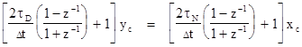
where the symbol z^–1 is the “past value” operator. For example, z^–1 y_c = y_p. Substituting equation (2.3.2-5) into equation (2.3.2-4), we have

Multiplying through by Δt(1+z^–1) gives

Rearranging terms, we have

Carrying out the indicated past value operations gives

Solving for y_c, we arrive at equation (2.3.2-2). Thus, when applied to a first-order transfer function, the bilinear substitution method gives the same recurrence formula as the method of finite differences. However, this is not the case for the second order functions, as is shown in Section 3.3.

2.3.3  Pre-Warping

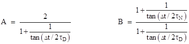
A technique called “pre-warping” is sometimes applied to lead/lag algorithms in an attempt to correct the amplitude of the output responding to an oscillating input signal. The standard recurrence coefficients for this method are

Recalling that as z goes to zero, tan(z) approaches z, we see that the pre-warped coefficients reduce to equations (2.3.2-3) if Δt is small relative to τ_N and τ_D.

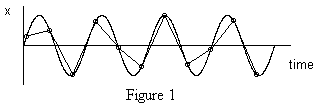
The rationale for pre-warping is clarified by the following example. Given a lead/lag simulation with time-step size Δt = 0.25 seconds and a sinusoidal input function with a period of T = 1 second, each cycle of the input will be described by four discrete values, as illustrated in Figure 1.

Clearly a sample will rarely be taken at an absolute peak of the wave, even if T is not an exact multiple of Δt and the samples precess through the cycle. Therefore, assuming linear interpolation between the discrete values, we will truncate most of the peaks and under-represent the true amplitude of the input function, which results in a corresponding underestimation of the output amplitude. In an attempt to correct for this, pre-warping biases the recurrence coefficients to reduce the effective lag of the filter, thereby increasing its output amplitude for a given oscillating input. However, the bias necessary to cancel out the under-representation of the input varies with the ration of T to Δt, so the pre-warped coefficients are really only correct for one particular frequency – by convention, the “half power frequency”. At lower frequencies, and for most non-oscillatory inputs, the pre-warping coefficients yield less accurate results than the approximate coefficients given by equations (2.3.2-3). Hence, pre-warping is a highly specialized technique, intended only for a limited range of frequency-response applications.

2.3.4  Composite Past Value Recurrence

All the solution methods discussed so far have assumed the availability of xp and yp, that is, past values of the input and out functions. This requires the dedication of two RAM memory locations for each lead/lag in the system. In contrast, the composite past value (CPV) recurrence scheme required only one stored value. In the constant-τ case this recurrence scheme is functionally equivalent to the standard recurrence formula for any given solution coefficients A and B. However, when CPV recurrence is applied in the variable-t case, it does not give exactly the same results as the standard formula.

To derive CPV recurrence formula, we begin by rewriting the standard formula as follows

Dividing and multiplying the two past-value terms by 1–B gives

If we define the quantity in the brackets as the “composite past value”, denoted by z_p, then we can rewrite equation (2.3.4-1) as

or

The composite current value is defined as

To simplify this, we substitute the expression for the y_c from equation (2.3.4-2), which gives

Combining terms in x_c and simplifying, we have

Therefore, the CPV recurrence formulas are

The derivation of these formulas does not distinguish between the past and current values of A and B, thereby tacitly assuming that these coefficients are constant. However, when τ_N and τ_D are variable, the standard coefficients A and B are also variable, in which case the CPV recurrence formulas are not exactly equivalent to the standard formula on which they are based. To demonstrate this, we can solve equation (82.3.4-3) for z_p and substitute this into equation (2.3.4-4) to give

A and B are now subscripted with a “c” to denote the current values, since only the current values are available each time the recurrence formulas are executed. Equation (2.3.4-5) is also valid at the past instant, which is to say

If we substitute this expression for z_p into equation (2.3.4-3), the resulting equation for y_c can be reduced to the form

where A_eff and B_eff are the effective standard recurrence coefficients, related to the actual coefficients used in the CPV recurrence formula by

Because of this effect, there are circumstances in which CPV recurrence yields unrealistic output response, even if the optimum formulas for A and B are used. The simplest illustration of this is the case where τ_N and τ_D initially have different values and then become equal. The true first order response is for the output to asymptotically converge on the input function once τ_N = τ_D, and this can be accurately simulated using the standard recurrence formula. However, this response cannot be reproduced using CPV recurrence. To understand why, notice that whenever τ_N = τ_D the current value of B (denoted by B_c) must equal 1, as is clearly shown by equation (2.2.3-4). Substituting this into equations (2.3.4-6) gives the effective coefficients A_eff = 1 and B_eff = 1. Inserting these into the standard recurrence formula gives the result

Thus, using CPV recurrence, the output undergoes a “step” change and “instantaneously” becomes equal to the current input, regardless of the output’s past value.

A possible objection to equation (2.3.4-1) is that it appears to predict divergent behavior when B_p equals 1, whereas in practice CPV recurrence formulas never yield divergent response. The explanation is that B_p can only equal 1 if B_c of the previous iteration was 1. But we have already seen that if B_c was 1 for the previous iteration, then y_c was unconditionally set equal to x_c during that iteration. Therefore, for the present iteration, y_p must equal x_p. Recalling that A is the coefficient (x_p – y_p) in the standard recurrence formula, we see that, in effect, the divergence of A_eff at B_p = 1 is always “cancelled” by the vanishing of (x_p – y_p).

2.3.5  Discussion

Digital simulations of continuous dynamic functions have a constraint on their execution frequency imposed by the intrinsic information rate of the input and output signals. The execution frequency must be high enough to resolve and convey the significant characteristics of these signals. However, the simplified methods of simulation described in Sections 2.3.1 and 2.3.2 have another limitation: The approximations on which they are based are valid only if the execution period Δt is small relative to the characteristic times of the function (i.e., τ_N and τ_D). To illustrate that these two limitations are logically independent, consider the simple lag response

where τ = 0.05 seconds. Equations (2.3.2-3) give the recurrence formula

Now suppose that, based on their maximum information rates, we have determined that x and y can be adequately represented with a sampling frequency of 4 Hz, corresponding to a  Δt  of 0.25 seconds. Substituting this into equation (2.3.5-1) gives

A sample of the response given by this recurrence formula for a single time-step is illustrated in Figure 2.

Figure 2

The output computed by equation (2.3.5-2) crosses over the input, which is obviously not representative of a pure lag response. In general, recurrence formulas based on equations (2.3.2-3) will not give an accurate representation of a lead/lag function unless Δt is less than 2τ. This means that the execution frequency of the present example would have to be raised from 4 Hz to at least 10 Hz. In contrast, if the optimum coefficients given by equations (2.2.3-4) are used, the recurrence formula is

for which an execution frequency of 4 Hz is adequate. Thus the use of non-optimal coefficients imposes unnecessarily high execution frequency on the simulation.

Another way of looking at this is to regard the error in the computed value of y_c for any given interval Δt as consisting of two parts: one part due to the uncertainty in the input function, and one part resulting from the approximations made in determining the coefficients of the recurrence formula. The first part is unavoidable (for a given Δt), but he second part can be eliminated entirely by using the optimum recurrence coefficients.

With the technique of pre-warping, an attempt is made to use these two errors to compensate for each other. However, as discussed in Section 2.3.3, these two errors offset each other only under a limited range of conditions. Essentially, pre-warping attempts to account for non-linearity in the input signal over the interval Δt, but there is really no general way of determining the non-linearity of a signal based on just two samples (x_p and x_c). In applying its “correction”, pre-warping makes use of information about the input signal beyond what can be inferred from the two given points. Specifically it depends on the knowledge that the input is periodic with a given frequency. Without such special information, a general method of accounting for non-linearity of the input signal must make use of at least three values of x. With three values we can determine the optimum recurrence formula based on second order interpolation of the input function. Denoting the “past past value” of x by x_pp, the expanded recurrence formula can be written

where

By the same reasoning that led to the relation f₁ + f₂ + f₃ = 1, we have the relation

Using this, we can re-write equation (2.3.5-3) in a generalized standard form analogous to equation (2.2.2-2) as follows

where

If x_pp, x_p, and x_c are co-linear vs time, then the quantity multiplied by C vanishes, and equation (2.3.5-4) reduces to equation (2.2.2-2).

Regarding the technique of CPV recursion, it is worth noting that the form developed in section 3.3 is not unique. Beginning with equation (2.3.4-0), we could have defined the composite past value directly as just the sum of the past value terms

Then the CPV recurrence formulas would have been

The advantages of equations (2.3.4-3) and (2.3.4-4) is that they can be executed with just two multiplications, whereas equations (2.3.5-5) and (2.3.5-6) involve three multiplications. This is significant because multiplication is a time-consuming operation in most digital devices. However, equations (2.3.5-5) and (2.3.5-6) will give better accuracy in the variable-τ case because they are equivalent to using the effective standard coefficients

These coefficients never yield singular values of the coefficients, unlike equations (2.3.4-3) and (2.3.4-4) when B_c=1, so no special provisions are needed to account for this computational singularity (recognizing that it cancels when multiplied by (x_c - x_p)).

Return to Table of Contents