Interference or Refraction?

1.0  Introduction

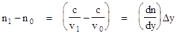
The index of refraction for a transparent medium is defined as n = c/v where c is the speed of light in vacuum and v is the speed of light in the medium. In a typical gas the index of refraction is related to density by

where k is a constant and ρ_ref is the density of the gas at a reference condition, typically 0C at 760 mm Hg. For air we have k = 0.000292, and ρ_ref = 0.041206 slugs/ft³, which equals 0.001702 kg/m³.

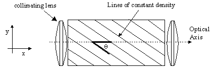
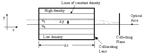
Suppose the air density in the test region varies linearly in a single direction, such that the lines of constant density (and refractive index) make an angle of θ with the axis of the optical beam, as illustrated below:

There are two different ways of conceptualizing how the non-uniform air density causes the distribution of energy incident on the receiver to vary. First, we can conceive of the optical rays being diverted in their course as they cross the test chamber, due to refraction resulting from the density gradient. This causes the rays to enter the downstream “de-collimating lens” at a slight angle to the optical axis, and therefore to be directed slightly away from the nominal focal point.

Second, we can consider the family of all possible linear paths across the test chamber (parallel to the optical axis), and note that a phase difference will exist between those paths, due to the variation in mean refractive index. According to this view, the nominal focal point for most of the optical energy of the device is the location of the primary interference fringe, where all the coherent light rays arrive in phase, assuming uniform density in the test chamber. If the density is non-uniform, the primary fringe (i.e., the point on the collector screen at which photons traveling along the different possible paths arrive in phase) occurs at a slightly different location.

These two interpretations are essentially equivalent, because the phenomenon of refraction is fundamentally a consequence of phase shift of different parts of a wave front, which can be regarded as effectively tilting the wave front, causing the light rays to be diverted. This tilting of the wave front consists of a shift in the phase of neighboring rays, which causes the point of maximum probability amplitude on the receiving screen to shift. Of course, the ray-tracing model with refraction considers only the primary fringe, whereas the quantum electrodynamics model with phase shift accounts for all the fringes.

2.0  Refraction Interpretation

To estimate the effect of a given density gradient in the test region on the nominal focal point of the device, we can consider the case where θ = 0, which means the lines of constant density are parallel to the optical axis (i.e., the x axis in the drawing above), and the density gradient is therefore perpendicular to the axis. The general equations of motion of a light ray in a medium of continuously varying refractive index are

                                  (1)

If the refractive index in a region is purely a linear function of y, it’s easy to verify that these equations are satisfied by a catenary curve, the general form of which is

y  =  k cosh(x / k)                                                        (2)

where the origin of the vertical parameter y is placed at the point where the curve is tangent to a line of constant density, and the constant k equals n₀ / (dn/dy), where n₀ is the refractive index at the tangent point, and dn/dy is the (constant) rate of change of the refractive index with respect to the y coordinate.

The slope of the light ray as the exit plane is given by

dy/dx  =  sinh(Δx / k)                                                  (3)

If we assume the angular deflection of the ray exiting the de-collimating lens is approximately equal to the deviation from the optical axis of the ray entering the lens, and that the axial distance from the lens to the collecting plane is x_f, it follows that the ray will be laterally shifted at the collecting plane by a distance of s = x_f Δx / k, which is

                                                 (4)

(Note that we’ve used the small-angle approximation sinh(x) ≈ x.) We will assume the test section has a length of Δx = 1 meter, and the focal length of the de-collimating lens is x_f = 0.05 meters. Also, the nominal index of refraction n₀ is assumed to be 1.000292, and the dependence of the refractive index on density ρ is given by

                                                             (5)

where K is a constant equal to 0.000292 for air, and ρ_ref is the density at the reference condition, which is ρ_ref = 0.041206 slugs/ft³ = 0.001702 kg/m³. In the test section we have assumed the density is just a linear function of y, so we have

                                                      (6)

Substituting this into the expression for n and differentiating on y gives

                                                       (7)

Consequently, the overall expression for the lateral shift in the light ray at the collector plane is

                                                 (8)

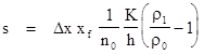
where ρ₀ denotes the density at the centerline (which we’ve taken as ρ_ref). Since the derivative of r with respect to y is assumed constant, we can put dρ = ρ₁ – ρ₀, where ρ₁ is the density at the “top” of the test region, and let dy = h (to signify the “height” of the test region above the centerline). In these terms we have

                                                 (9)

To express this in terms of variations in total pressure, rather than density, we can substitute based on the relevant thermodynamic relations (see the Appendix) to give

                                        (10)

If the total pressure varies by 10% from one region of the inlet to another, we may assume that the total pressure from the centerline to the top of the test region varies by 5%, so the ratio p_t1/p_t0 equals 1.05. Inserting this along with the values of the other variables in the above formula gives the result 0.41 microns.

3.0  Interference Interpretation

An alternative way of conceptualizing the effect of non-uniform air density on the focal point of the collimated beam is in terms of the interference between the rays passing through different regions of air.

The phase velocity of light in the medium is inversely proportional to the refractive index, i.e., we have n = c/v, where c is the speed of light in a vacuum. We have

                                (11)

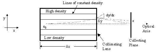
Since the time required for a ray of light to traverse the test region is Δx / v, it follows that the upper path of light shown in this figure is phase-delayed relative to the center ray by an amount of time equal to

                                      (12)

The primary constructive interference fringe must therefore be located on the collecting plane at a point so as to offset this time lag, i.e., at the point which the two rays will reach simultaneously in phase. We assume the de-collimating lens corrects for the nominal offset between the rays, so that if n₁ = n₀ the primary fringe would be precisely on the optical axis. We need to determine the lateral shift in the focus point that lengthens the center ray and shortens the upper ray by a combined amount equal to the time lag noted above.

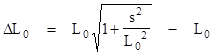
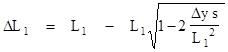
From the de-collimating lens to the collector screen the central ray nominally travels a distance of L₀ = x_f, and the upper nominally travels a distance given by L₁² = x_f² + Δy². If the focus point shifts in the positive y direction by a distance s, the central beam will travel a slightly greater distance, denoted by L₀ , and the upper beam will travel a slightly lesser distance, denoted by L₁. This shift will compensate for the different air densities in the test region if the combined change in travel times equals the value of Δt₁ – Δt₁ noted above. The shifted distances are given by the relations

L₀  =  x_f²  +  s² L₁  =  x_f²  +  (Δy – s)²

If we define ΔL₀ = L₀ – L₀ and ΔL₁ = L₁ – L₁, then we have

Now, since the shift s is extremely small in comparison with L₀ and L₁, we can closely approximate the square roots by their first order expansions, which give

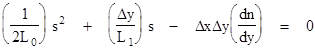
Equating the sum of these increments to the effective distance corresponding to the time lag derived above, we have

                             (13)

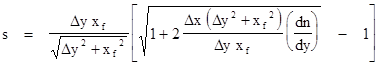
Solving this quadratic for s gives

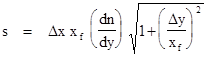
Since the constant dn/dy is extremely small, the second term under the square root is much less than 1, so we can use the first-order expansion to give

                                            (14)

Substituting for dn/dy from the same thermodynamic considerations as in the refractive analysis, we arrive at a predicted shift of

                                      (15)

4.0  Discussion

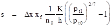
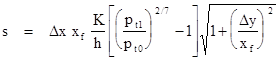
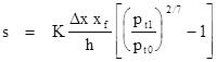
Notice that the square root factor in (15) is on the order of 1 (and approaches 1 as the half-width Δy of the beam goes to zero), and the factor 1/n₀ in equation (10) is also nearly equal to 1 (since the case we’ve been considering has assumed that n₀ differs only slightly from unity). Therefore, both the refractive and the interferometric approaches predict a shift of the focus point by a distance s on the order of

where K = 0.000292 (dimensionless) for air, Δx is the length of the test region, x_f is the focal length from the de-collimating lens to the collector plane, and h is the lateral distance over which the total pressure in the test region changes from p_t0 to p_t1.

The slight differences between (10) and (15) are not surprising, because our interference analysis was arbitrarily based on just two specific paths, separated laterally by a distance of Δy, whereas the refraction analysis was based on a single ray of infintesimal width beginning from the optical axis. Thus we expect to find a factor in the interference solution that goes to 1 as the path separation Δy goes to 0. Also, the factor of 1/n₀ that appears in the refractive solution is excluded from the interference solution only because of the approximations that were made in the latter, based on the premise that n₀ is nearly equal to 1. Hence the effect can be modeled equally well as refraction or as interference, assuming we are interested only in the dominant primary fringe. In order to predict the behavior of the higher-order fringes it would obviously be necessary to apply the interference analysis.

Appendix

For an ideal gas the static pressure, temperature, and density (denoted by p, T, and ρ) are related by the equation p = ρRT. Also, the total (stagnation) temperature and pressure are related to the static temperature and pressure and the local Mach number according to the relations

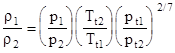
where g is the ratio of specific heats (7/2 for air). Combining these equations gives the following relation between the thermodynamic variables for any two conditions

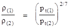
For adiabatic flow of a perfect gas the total temperature along any streamline (regardless of any increase in entropy) is constant, so we will set T_t(2)/T_t(1) = 1. Also, assuming the static pressures of all the streamlines at a given axial location are in equilibrium, we can set p₍₁₎/p₍₂₎ = 1. On this basis, we can estimate that the total pressure of two streamlines at the fan face are related to the densities at those locations by

For example, if a compressor has 10% distortion, then at the limiting condition there are streamlines whose total pressures at the fan face are in the ratio 1.1, which implies that the corresponding densities are in the ratio 1.027.

Return to MathPages Main Menu