Frequency Response of First-Order Lag

A first-order lag relation is often used to represent the dynamic response characteristics of simple systems. For any input signal x(t) the output signal y(t) satisfies the ordinary differential equation

where τ is the "time constant" of the response. If we set the input signal x(t) to a simple sine wave, the steady-state output signal y(t) will also be a sine wave, although the amplitude and phase of the signals will generally be different. One way of describing a first-order lag is in terms of the amplitude and phase differences it produces for sinusoidal input signals of various frequencies. Consider the response to an input signal given by

where A is the constant amplitude and ω is the constant frequency in radians per second. (The is equivalent to the frequency f = ω/2π expressed in cycles per second, also known as Hertz.) We surmise a steady-state solution of the form

where k is the amplitude gain factor, and θ is the phase shift between the input and output signals. The derivative of y(t) is

Substituting into the equation (1) gives

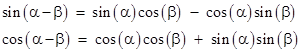
The constant A can be canceled out, and we can use the trigonometric identities

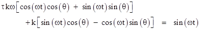
to expand the above equation into

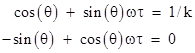
Equating the total coefficients of cos(ωt) and sin(ωt) on both sides of this equation and dividing through by k gives the two conditions

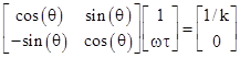
This is just a plane rotation through the angle θ, and can be written in matrix form as

Since a rotation doesn't change the length of the vectors, we must have

and so the amplitude factor k is given by

Also we can easily solve for the angle θ by dividing the equation –sin(θ) + cos(θ)ωτ = 0 through by cos(θ) to give tan(θ) = ωτ, from which we get

The expression for k shows that the amplitude of the output signal is the square root of a "Cauchy distribution" of the scaled input frequency ωτ. Typically we disregard negative frequencies, and we say this is a "low pass filter", because for small values of ωτ the amplitude factor k is nearly 1 (i.e., very little attenuation of the input signal), whereas for larger values of ωτ the amplitude factor drops. Likewise the phase lag is small when the frequency ωτ is low, but it increases as the frequency increases. Of course, the inverse tangent is a multi-valued function, and we typically just take the value from the principle branch in the range from 0 to π.

As an aside, notice that if we set the time constant τ equal to i (the square root of –1) and if we identify the frequency ω with the "velocity" v of a moving object, we get

Hence the amplitude factor of this transfer function equals the "gamma" factor of time dilation and length contraction in special relativity, and the phase angle is proportional to the additive "rapidity" corresponding to the velocity v. The differential equation (1) in this case may be written as

It's also interesting to compare this with the time-dependent Schrödinger equation

where h is the (reduced) Planck constant, H is the Hamiltonian operator for the system, and ψ is the quantum wave function of the system. If we identify the output signal y(t) of our filter with the wave function ψ(t) of the system, and if we identify (x–y)/h  with the scaled Hamiltonian operator of the system, then the correspondence between these equations is exact. Does this suggest an approach to a quantum mechanical description of spacetime?

Return to MathPages Main Menu