|
A Removable Singularity in Lead-Lag Coefficients |
|
|
|
As discussed in section 2.2.4 of Lead-Lag Algorithms, a recursive simulation of a first-order lead-lag transfer function |
|
|
|
|
|
|
|
can be written in the form |
|
|
|
|
|
|
|
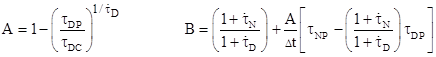
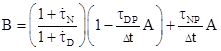
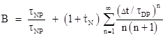
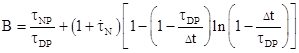
where the subscripts "c" and "p" denote current and past values respectively. If the time constants τD and τN are variable, and vary linearly over each time increment Δt, then the coefficients of the recurrence can be written as |
|
|
|
|
|
|
|
where |
|
|
|
|
|
On the surface it may
appear that B is infinite when |
|
|
|
|
|
|
|
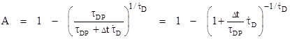
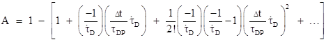
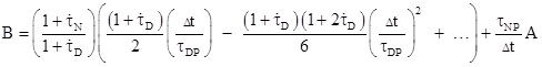
Assuming |
|
|
|
|
|
|
|
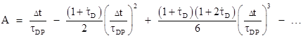
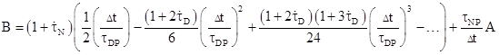
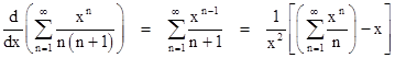
Extending the series and simplifying, we have |
|
|
|
|
|
|
|
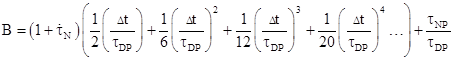
We now re-write B in the form |
|
|
|
|
|
|
|
Notice that as |
|
|
|
|
|
|
|
We can therefore cancel a
factor of |
|
|
|
|
|
|
|
Now, setting |
|
|
|
|
|
|
|
Thus when |
|
|
|
|
|
|
|
Note that the original
restriction |
|
|
|
|
|
|
|
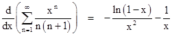
The summation in the right hand expression is the series expansion of −ln(1−x), so we have |
|
|
|
|
|
|
|
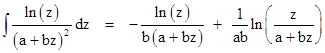
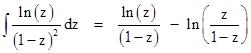
Making use of the well-known integral |
|
|
|
|
|
|
|
with a = −b = 1, we have |
|
|
|
|
|
|
|
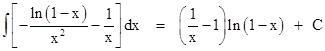
and therefore setting z = 1 − x (which gives dz = −dx) we arrive at |
|
|
|
|
|
|
|
Combining this with the 1/x term in the derivative of our infinite sum, and simplifying, we have the overall integral |
|
|
|
|
|
|
|
where the constant of integration is determined by the fact that our original summation vanishes as x = 0, and noting that the product (1/x − 1)ln(1 − x) goes to −1 as x goes to zero. Thus our summation can be written in closed form as |
|
|
|
|
|
|
|
Therefore, in terms of our
original problem, the singularity in B when |
|
|
|
|
|
|
|
which was to be shown. |
|
|