Aliasing and Uncertainty

The well-known phenomenon of "aliasing" in digital signal processing leads to an interesting uncertainty principle for certain pairs of conjugate parameters. Suppose we sample a continuous signal once every T = 0.05 seconds, i.e., our sampling rate is 20 Hz. In order to determine the derivative of this signal, we need to compare the values of the signal for at least two samples. If we let s[t] denote the sampled value of the signal at the time t, then a simple estimate of the derivative ds/T at the time kT is given by

However, we can't associate the value of the derivative with any specific instant. The mean value theorem from calculus assures us that at some instant in the interval from (k-1)T to (k)T the slope of the smooth function s(t) equals this value, but we are not able to specify where in this interval the slope has this value.

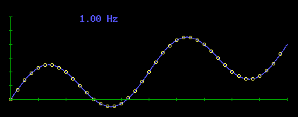
So far we've assumed our measurements of s[t] are exact, but suppose we superimpose a "noise" variability on top of the underlying signal. Let the noise be represented by a simple sinusoidal wave N(t) = h sin(ωt) where h is the amplitude and ω is the frequency of the noise. If the frequency of the noise is low relative to our sampling frequency, we will clearly resolve the wave pattern of the noise on top of a simple linear ramp signal s(t) = 2t + s₀ as illustrated below for a noise frequency of 1 Hz.

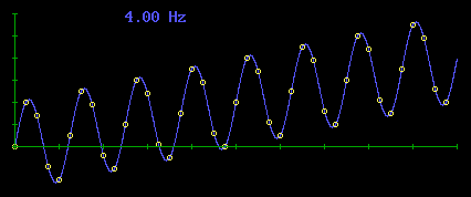
The discrete samples, even without the underlying blue curve, clearly show the fundamental wave pattern. However, if the noise frequency is somewhat higher, the coherence of the sampled profile is obscured somewhat, as shown below for a noise frequency of 4 Hz.

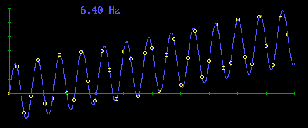
It would be difficult to discern the underlying blue curve (or any other simple curve) purely from the discrete samples. At a noise frequency of 6.4 Hz we could easily interpret the total input (signal plus noise) as a mixture of three distinct sine waves as shown by focusing on just the discrete samples in the figure below:

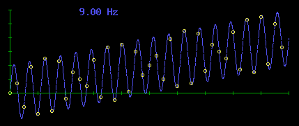
With a noise frequency of 9 Hz the total input appears as a mixture of just two sine waves in complementary phase as shown by the pattern of discrete samples below:

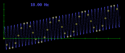
If we raise the frequency of the noise up to 18 Hz, so that it begins to approach the sampling frequency, the discrete samples appear as just a single sine wave as shown below:

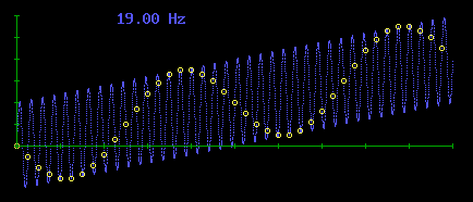
The frequency of this apparent sine wave is very dependent on the relation between the frequency of the noise and the sampling frequency. If we raise the noise frequency just one more Hz we find the total apparent frequency has been reduced, as shown below:

Naturally if the period of the noise is precisely equal to the sampling frequency, then we will always be sampling from the same phase of the noise, i.e., the same point on the wave form, so it will not contribute any oscillation to the input, although it may contribute a "DC" offset with a magnitude equal to anything up to the full amplitude of the noise.

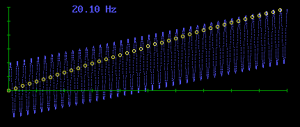
By matching the frequency of the noise arbitrarily close (but not exactly equal to) the sampling frequency we can produce a total input sequence that exhibits an aliased version of the noise equal to A sin(Ωt) where A is the same as the amplitude of the actual noise signal and Ω is the aliased frequency, which may be made arbitrarily small. To illustrate, here is the resulting total input with a noise frequency of 20.1 Hz:

The phenomena of aliasing provides an interesting illustration and interpretation of the difference between a superposition and a mixture. A superposition of two signals a(t) and b(t) is typically defined as just the sum a(t) + b(t). On the other hand, a mixture of these two signals is more subtle, since we are effectively partitioning the samples of a given total sequence into interlaced subsequences, each of which is interpreted or represented as a separate component. The distinction is that these components are not added together (as in a superposition), but rather we take the union of the samples.

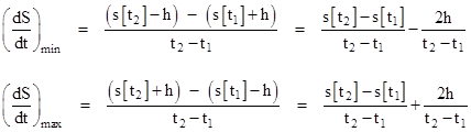
Returning to the original question, it's easy to see that the presence of sinusoidal "noise" with a fixed known amplitude h and unknown frequency ω places restrictions on how precisely we can determine the slope of the underlying signal. Since the aliased frequency of the noise can have any arbitrarily low frequency, any attempt to filter out the noise must be based on averaging the sampled values over a large number of samples. It's always possible for the total sequence S(t) = s(t) + N(t) to begin at the low end of the noise band and end at the high end (or vice versa) during the sequence of samples used to evaluate the derivative. Hence, assuming a basic ramp input signal with constant derivative, our estimate of the derivative based on the samples from any interval t₁ to t₂ can be anything between the two values

Consequently, if we let Q denote the derivative of s with respect to t, then the range of uncertainty in Q cannot be less than

Obviously for any fixed noise amplitude h we can reduce the uncertainty in the derivative Q to arbitrarily small values simply by increasing the sampling time Δt, but of course this assumes Q isn't changing during the period, and it increases the range of uncertainty on t, i.e., on precisely when the derivative actually had the computed value. Thus we have a familiar hyperbolic relationship between the uncertainties in Q and t, namely

In a sense we could regard t and Q as conjugate observables. In fact, if we map the time values t₁ and t₂ to the nominally corresponding signal values s(t₁) and s(t₂), then we have Δs ~ Δt, and so since Q is just ds/dt, we could identify s with spatial position and Q (multiplied by the constant m) with momentum, and we have the uncertainty relation

which is formally identical to Heisenberg's uncertainty relation in quantum mechanics. The same sort of relation applies to any pair of conjugate (non-commuting) observables. Of course, we shouldn't try to press an analogy like this too far, but this shows how signal processing provides an interesting model for hyperbolic uncertainty relations.

Return to MathPages Main Menu