Curvature of Linear Interpolation

Most people are familiar with linear interpolation applied to a two-dimensional table that gives discrete values of some function z = f(x,y) at discrete values x_n, y_n. Given a specific pair of coordinates x,y where  x₁ < x < x₂ and  y₁ < y < y₂  we interpolate using the four nearest table points shown below:

In spite of its simplicity, the surface of interpolation (i.e., the locus of interpolated points x,y,z) can be used to illustrate some interesting aspects of differential geometry. 

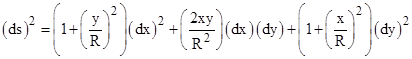
By a simple translation of the xyz coordinates the equation of this surface becomes simply z = xy/R where R is a constant, and the metric line element is

Thus the components of the metric are

The determinant of the metric at any point (x,y) is g = 1 + (r/R)² where r = (x² + y²)^1/2, and the intrinsic curvature is

Since the curvature depends only on r, this shows that the lines of constant curvature are circles when projected onto the xy plane. The parametric equations of geodesics on this surface are

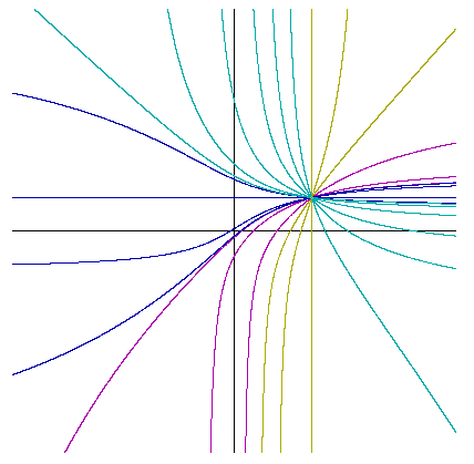
This shows that if either dx/ds or dy/ds equals zero, then the second derivatives of x and y with respect to s must be zero, which means that lines of constant x and lines of constant y are geodesics. Of course, loci that are not parallel to either the x or the y axis can also be geodesics, provided they satisfy the above equations. The plot below shows the family of geodesics through an arbitrary point on the surface.

Some of these loci proceed from one vertical asymptote to another, or from one horizontal asymptote to another, while other loci proceed from a vertical to a horizontal asymptote or vice versa. The boundary trajectories between these types can extend along diagonal asymptotes for arbitrary distances.

Return to MathPages Main Menu