Isospectral Point Sets in Higher Dimensions

A given configuration of n points in space determines a multi-set of n(n−1)/2 point-to-point separations, refered to as the distance spectrum of the configuration. The distance spectrum is physically significant because it represents the energy partition of a configuration of particles whose potential energy is strictly a function of the distances between particles. For example, the potential energy associated with two electrically charged particles due to the Coulomb force is proportional to 1/r, where r is the distance between the particles. The total potential energy of a collection of n particles is therefore partitioned into a multi-set of n(n−1)/2 contributions distributed according to the distance spectrum. Related to this is the fact that when a small cluster of particles (such as atoms in a molecule) are subjected to radiation, the spectrum of absorption and re-emission depends on the pairwise distances between the particles, because these distances characterize the energy modes of the cluster.

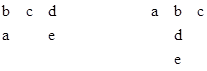
Although a given geometrical configuration of particles has a definite distance spectrum, the mapping between configurations and distance spectrums is not one-to-one. It’s possible for geometrically distinct arrangements of particles to have the same distance spectrum, in which case the arrangements are said to be isospectral. One-dimensional isospectral configurations are discussed in Generating Functions for Point Set Distances. There also exist such arrangements in two or more dimensions. For example, given the multi-set of ten separations

we can construct either of the two five-point configurations shown below

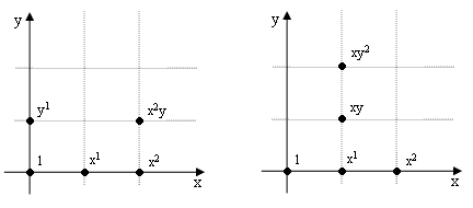
Naturally translations, rotations, and reflections have no effect on the intrinsic distances between the points of a given configuration, and we know the familiar invariants associated with transformations of these kinds. To find an invariant for more general transformations, including the one that maps between the two arrangements shown above, we can begin by encoding each square lattice arrangement as a polynomial in variables x and y, with exponents denoting the coordinates in the horizontal and vertical directions respectively. First we place the two configurations on a lattice as shown below

We can then read off the corresponding polynomials

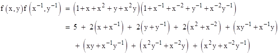
For any such polynomial, a generating function for the point-to-point distances of the corresponding point set is given by the product of f(x,y) and f(1/x,1/y), since this effectively gives a polynomial with exponents equal to the differences in the exponents of the original polynomial. However, each distance (except for the null distances from each point to itself) is counted twice, as a reciprocal pair of terms. For example, the ten non-null distances for the left-hand configuration above can be read from the product

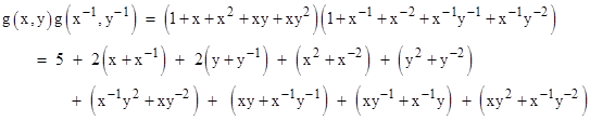
Each of the 25 point-to-point distances can be recognized in this last expression. The constant “5” represents the five null distances from each of the five points to itself. Carrying out the same procedure for the other configuration gives

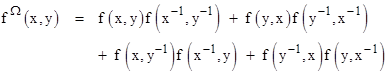
As would be expected, many of the terms are common between this and the previous expression, but not all. The discrepancies are due to the two possible orientations for each separation, corresponding to the transposition xy to yx. To give an invariant expression, we need to add the product twice, with both possible permutations of x and y. In the case of the two simple configurations above, this would be sufficient, but in general for larger and more complex configurations we need to also account for differences parity by including mixed terms for x,y⁻¹ and y⁻¹,x. Thus for any polynomial f(x,y) representing a configuration of points on a 2-dimensional orthogonal lattice, the polynomial f ^Ω(x,y) defined by

is an invariant indicator of the multi-set of point-to-point distances. Of course, it is invariant under translations, lattice rotations, and reflections, as well as under transformations from one configuration to any isospectral configuration. (If desired we can clear the fractions from this function by multiplying through by x and y raised to the powers of their respective degrees in f.) We often regard two configurations of points as “the same” (i.e., equivalent) if they can be superimposed by a coherent translation, rotation, or even reflection. These operations preserve not only the intrinsic point-to-point distances (and therefore the energy partition) of the configurations, but also the identities of the particles at the terminals of those distances. If we relax the latter requirement, so that the identities of the particles are not necessarily maintained, we get a larger sense of equivalence that regards two configurations as “the same” if they are isospectral. (It’s worth noting that in quantum mechanics the wave functions of a collection of particles overlap, so the individual identities of the particles from one observation to another are not definite.)

It is straightforward to confirm algebraically that the polynomials f and g yield the same indicator polynomial, and this can be corroborated numerically by substituting particular values for x and y into these expressions and noting the equality of the results. For example, arbitrarily assigning the values x = 3, y = 7, we can easily compute

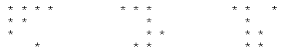
For another example, consider the following three distinct configurations of eight points, each of which has the same multi-set of 28 point-to-point separations:

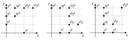
Placing these configurations on an orthogonal lattice, we can assign polynomial terms to each of the points as shown below.

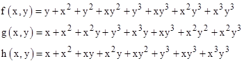
Thus the polynomials corresponding to these three configurations are

To confirm that these three configurations are isospectral we need only show that their indicator polynomials are identical. This can be shown algebraically, and we can corroborate the finding numerically, by arbitrarily inserting values of x = 2,y = 3 into the indicator polynomials, giving

Incidentally, of the 12870 possible arrangements of eight points on a 4x4 orthogonal grid, there are only 1120 different sets of separations. Of course, much of this reduction is due to rotations and reflections, but not all. Configurations with unique distance spectrums are evidently exceptional.

We can generalize the above approach to deal with lattice configurations of points in any number of dimensions. For example, in three dimensions we would encode each configuration as a polynomial f(x,y,z) in three coordinates, and then the indicator polynomial f ^Ω(x,y,z) must account for all six possible permutations of the coordinates as well as for the four possible combinations of signs. There are actually 2³ = 8 possible combinations of the three signs, but we get a complimentary pair of these for each product term in the definition of the indicator polynomial. Thus the indicator polynomial in three dimensions is defined as the sum of 24 products of two of the f functions with complimentary arguments. In general the indicator polynomial for n-dimensional configurations of lattice points consists of 2ⁿ⁻¹n! terms, so for 1, 2, 3, 4, and 5 dimensions the number of terms is 1, 4, 24, 192, and 1920 respectively.

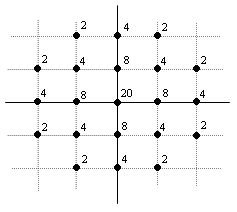
The indicator polynomial f ^Ω for any given point-set polynomial f can also be regarded as a point-set polynomial of the same degree as f. For example, the indicator polynomial for the point-set corresponding to f(x,y) = 1 + x + x² + y + x²y can be interpreted as the point set shown below. (The integers next to each node indicate the number of particles located at that point.)

This could lead to a higher-order equivalence relation, because it’s conceivable that two point sets represented by the polynomials f and g might have distinct indicators f ^Ω and g^Ω, and yet the indicators of these polynomials, denoted by (f ^Ω)^Ω and (g ^Ω)^Ω, might be identical. It would also be interesting to investigate the asymptotic distribution of particles under repeated iterations of the indicator transform.

Return to MathPages Main Menu