|
Ratio Populations |
|
|
|
|
|
|
|
|
|
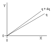
If we take a random sample from X and a random sample from Y, the combined sample {x,y} is a point on this plane. Of course, the joint density function for the point (x,y) is simply the product of the two univariate densities g(x)h(y), and the probability of a random joint sample falling within any particular region is just the integral of g(x)h(y) over that region. |
|
|
|
The line labelled "q" is the set of all points for which the ratio y/x equals the constant q. To find the probability that a random sample would give a ratio less than q, simply integrate g(x)h(y) over the region of the plane below the line, i.e., |
|
|
|
|
|
|
|
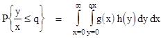
Similarly, we can compute the incremental probability of the ratio y/x being between q and q+dq for some small constant increment dq. This is just |
|
|
|
|
|
|
|
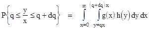
Of course, g(x) is independent of y, so we needn't place it within the "inner" integral. Also, notice that if we choose dq small enough the value of h(y) will be virtually constant because y will be essentially equal to qx. Thus we can move both g(x) and h(y) outside the inner integral and set h(y) = h(qx) to give |
|
|
|
|
|
|
|
|
|
This quantity is called "d F(q)" because it's the incremental change in the cumulative distribution function F(q) for an incremental change dq in the ratio. |
|
|
|
Now we just need to evaluate the square brackets, which is easy because the integral of dy is just y, and evaluating this from y = qx to (q+dq)x gives simply x dq. Making this substitution and dividing both sides by the constant increment dq gives the density function |
|
|
|
|
|
|
|
In the limit as dq ® 0 this becomes the exact derivative of the cdf F(q) with respect to q, so this is the density function f(q) for the ratio population Y/X. |
|
|
|
For "two-sided" distributions (i.e., distributions with positive density on both sides of zero) the joint state space covers the whole plane, instead of just the first quadrant, but the derivation is essentially the same. We just extend the incremental "slice" through the origin into the negative region. The only change needed in the formula is to use the absolute value of x (because the q and q+dq lines are "flipped over" in the 3rd quadrant). Thus the general formula for ratio densities is |
|
|
|
|
|
|
|
where h is the numerator density and g is the denominator density. Interestingly, it turns out that if h and g are normal distributions with negligible density at 0, then the above integral for f(q) has a closed-form expression in terms of elementary functions. Even without the requirement for negligible densities at 0 we can express f(q) in terms of the error function. |
|
|
|
Given two normally distributed populations A and B with means μA and μB and standard deviations σA and σB, we consider the population C each of whose members consists of the ratio of randomly selected samples from A and B. If the populations A and B such that essentially all of their elements lie on the same side of zero (i.e., if their means are more than, say, six times their standard deviations), then the distribution density of the C population is essentially |
|
|
|
|
|
|
|
This isn't a normal distribution, but the integral is fairly well behaved as long as the B population doesn't have significant density at zero, in which case C has a fairly well-defined "pseudo mean" and "pseudo standard deviation", defined by truncating the usual integrals at some finite limit where the density falls below some arbitrarily small level. |
|
|
|
However, strictly speaking, if B has positive density at zero, the ratio population has a "Cauchy" component, and the mean and standard deviation are undefined (the integrals diverge). This is because some of the elements of C are undefined (i.e., non-zero elements of A divided by a zero element of B). |
|
|
|
Even in the case where the density of B vanishes at zero, the original question is still under-defined, because the means and variances of A and B are not sufficient to determine the mean and variance of C. We have to deal with the complete distribution characteristics, because we can get very different answers for the same means and standard deviations just by reshaping the distributions. |
|
|
|
Assuming A and B are normal with nearly vanishing densities at zero, the distribution density of C is as given by equation (1), which has the closed form expression |
|
|
|
|
|
|
|
This reveals some interesting facts. For example, we might think that the pseudo mean of the distribution of ratios A/B would be just the ratio of the means μA/μB, but that's not the case. The median of the C distribution is approximately equal to the ratio of the means, but typically the pseudo-mean of the C distribution is different. |
|
|
|
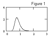
To illustrate, suppose A is a normal population with mean of μA = 90 and standard deviation of σA = 12, and suppose B is a normal population with mean of μB = 110 and standard deviation of σB = 20. The median of the distribution of ratios of elements of A divided by elements of B is equal to 90/110 = 0.818, but the pseudo-mean of the distribution is 0.848. The maximum density of the distribution occurs at 0.76977. The pseudo standard deviation of the distribution is 0.21. A plot of the C density distribution for this case is shown in Figure 1. |
|
|
|
|
|
|
|
If we consider the special
case of ratios consisting of two elements drawn from a single normally
distributed population with mean μ far from zero (relative to the unit
standard deviation), then the distribution of the ratios approaches normality
with mean 1 and standard deviation |
|
|
|
|
|
|
|
If we change variables by putting t = r + 1, then the r = 0 point maps to the t = 1 point, and we have |
|
|
|
|
|
|
|
Expanding this around the r = 0 point gives |
|
|
|
|
|
|
|
This is the normal
distribution with mean r = 0 (which, remember, is t = 1) and standard
deviation of |
|
The preceding discussion has focused on cases where the elements of B were essentially all non-zero. It's interesting to consider what the distribution of ratios would be for populations that had significant densities at zero. For example, what would the C density look like if A and B were standard normal distributions with means equal to zero? The answer for the general case is given by the same integral as in Equation 1 above, except that the "x" in the integral is changed to the absolute value of x, as follows: |
|
|
|
|
|
|
|
Now it's applicable to any two normal populations A and B, with positive, negative, or zero means. The only caveat is that the integral no longer has a simple closed-form expression in terms of elementary functions. However, in terms of the error function erf(x) the C density in the general case can be expressed as |
|
|
|
|
|
where |
|
|
|
|
|
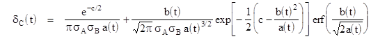
This formula gives an interesting range of distributions for various choices of the parameters for the A and B populations. For example, if A and B are standard normal populations with means of zero and standard deviations of 1, then b(t) = c = 0 and a(t) = 1+t2, so the density distribution of the ratio population is just the "Cauchy distribution" |
|
|
|
|
|
|
|
which happens to be identical to the asymptotic distribution of the iterates of certain linear fractional transformations. A plot of this is shown in Figure 2. |
|
|
|
|
|
|
|
The Cauchy distribution does not have a well-defined mean or variance (or standard deviation), because the variance integral doesn't converge, nor does the mean integral. This explains why, strictly speaking, no ratio density has a well defined variance, because the first term in the general expression for the density always contributes a "Cauchy component" to the variance integral, preventing it from converging. The only reason we can (seemingly) compute a mean and variance for the ratio distribution shown in Figure 1 (i.e., when the A and B means are far from zero) is that the Cauchy term is microscopic and it's easy to neglect it with a clear conscience. |
|
|
|
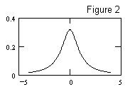
Now for a few interesting examples. Suppose the A population has a mean of 20 and a standard deviation of 1, and suppose the B population has a mean of 0.5 and a standard deviation of 1. The density of the ratios is shown in Figure 3. |
|
|
|
|
|
|
|
Since the B population has significant density at 0, the Cauchy term is fairly large, as can be seen from the fact that the tails of the curve do not drop off exponentially. The variance of this population is strictly undefined. Also, notice that the ratios really come in two distinct populations, viz., positive and negative (because the B population straddles zero). |
|
|
|
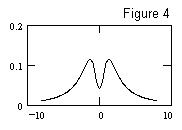
To make a symmetrical distribution, set the mean of A to 2, and the mean of B to 0. Then the ratios have the distribution shown in Figure 4. |
|
|
|
|
|
|
|
As we move the mean of A closer to 0, the "valley" between the two peaks gets smaller and smaller. When the mean of A equals 1, the top is flat like a plateau. When the mean of A gets to zero, we're back to the pure Cauchy distribution. |
|
|
|
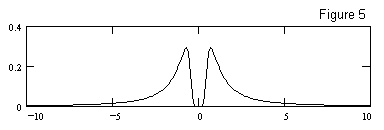
One more example. What is the distribution of the inverse of a standard normal population? To find this, we give A a mean of 1 with a standard deviation of 0 (so every element of A is exactly equal to 1). Then we set the mean of B to 0 and the standard deviation to 1. The resulting population of ratios (where each element is just the inverse of an element of B) is shown in Figure 5. |
|
|
|
|
|
|
|
It might seem surprising that the formula doesn't "blow up" as σA goes to 0, since σA appears in the denominator of some terms. However, it is also in the numerator, so it is a "removable" singularity. |
|
|
|
So, the distribution of ratios of two normal distributions does not, in general, have a well-defined variance (or mean, for that matter). However, if we restrict ourselves to just populations far from zero (i.e., populations that have no significant density at zero), then we can use equation (2), which neglects the Cauchy term, to define a pseudo mean and variance for the ratio distribution, as shown in Figure 1. |
|
|
|
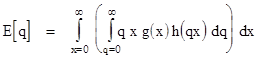
If our interest is solely in the expected value (i.e., the mean) of a ratio population, we can derive a simple result from equation (0), provided the denominator density g(x) vanishes at x = 0. Recall that the density distribution of the ratio population q = y/x is |
|
|
|
|
|
|
|
It follows that the expected value of q is |
|
|
|
|
|
|
|
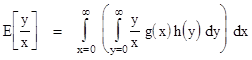
Swapping the order of the integrations, this can also be written as |
|
|
|
|
|
|
|
For the interior integral the value of x is a constant, and since y = qx, we see that y ranges from 0 to infinite as q ranges from 0 to infinity, and we have dy = x dq. Hence we can replace q with y/x, and x dq with dy, and change the interior integral to range over the y variable, giving |
|
|
|
|
|
|
|
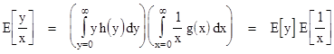
We can separate the integrand into functions of x and functions of y, and since they are independent we can write the double integration as the Cartesian product of two single integrations, which gives the result |
|
|
|
|
|
|
|
The quantity E[y] can be regarded as the arithmetic mean A[y] of y, and the quantity E[1/x] can be regarded as the reciprocal of the harmonic mean H[x] of x, so this last result is sometimes expressed in the form E[y/x] = A[y] / H[x]. |
|
|